nvdiffrast

Modular Primitives for High-Performance Differentiable Rendering

Table of contents

Overview

Nvdiffrast is a PyTorch/TensorFlow library that provides high-performance primitive operations for rasterization-based differentiable rendering. It is a lower-level library compared to previous ones such as redner, SoftRas, or PyTorch3D — nvdiffrast has no built-in camera models, lighting/material models, etc. Instead, the provided operations encapsulate only the most graphics-centric steps in the modern hardware graphics pipeline: rasterization, interpolation, texturing, and antialiasing. All of these operations (and their gradients) are GPU-accelerated, either via CUDA or via the hardware graphics pipeline.

Modular Primitives for High-Performance Differentiable Rendering
Samuli Laine, Janne Hellsten, Tero Karras, Yeongho Seol, Jaakko Lehtinen, Timo Aila
ACM Transactions on Graphics 39(6) (proc. SIGGRAPH Asia 2020)

Paper: http://arxiv.org/abs/2011.03277
GitHub: https://github.com/NVlabs/nvdiffrast

Examples of things we've done with nvdiffrast

Installation

Minimum requirements:

• Linux or Windows operating system.
• 64-bit Python 3.6.
• PyTorch (recommended) 1.6 or TensorFlow 1.14. TensorFlow 2.x is currently not supported.
• A high-end NVIDIA GPU, NVIDIA drivers, CUDA 10.2 toolkit.

To download nvdiffrast, either download the repository at https://github.com/NVlabs/nvdiffrast as a .zip file, or clone the repository using git:

git clone https://github.com/NVlabs/nvdiffrast

Linux

We recommend running nvdiffrast on Docker. To build a Docker image with nvdiffrast and PyTorch 1.6 installed, run:

./run_sample.sh --build-container

We recommend using Ubuntu, as some Linux distributions might not have all the required packages available. Installation on CentOS is reportedly problematic, but success has been claimed here.

To try out some of the provided code examples, run:

./run_sample.sh ./samples/torch/cube.py --resolution 32

Alternatively, if you have all the dependencies taken care of (consult the included Dockerfile for reference), you can install nvdiffrast in your local Python site-packages by running

pip install .

at the root of the repository. You can also just add the repository root directory to your PYTHONPATH.

Windows

On Windows, nvdiffrast requires an external compiler for compiling the CUDA kernels. The development was done using Microsoft Visual Studio 2017 Professional Edition, and this version works with both PyTorch and TensorFlow versions of nvdiffrast. VS 2019 Professional Edition has also been confirmed to work with the PyTorch version of nvdiffrast. Other VS editions besides Professional Edition, including the Community Edition, should work but have not been tested.

If the compiler binary (cl.exe) cannot be found in PATH, nvdiffrast will search for it heuristically. If this fails you may need to add it manually via

"C:\Program Files (x86)\Microsoft Visual Studio\...\...\VC\Auxiliary\Build\vcvars64.bat"

where the exact path depends on the version and edition of VS you have installed.

To install nvdiffrast in your local site-packages, run:

# Ninja is required run-time to build PyTorch extensions
pip install ninja

# Run at the root of the repository to install nvdiffrast
pip install .

Instead of pip install . you can also just add the repository root directory to your PYTHONPATH.

Primitive operations

Nvdiffrast offers four differentiable rendering primitives: rasterization, interpolation, texturing, and antialiasing. The operation of the primitives is described here in a platform-agnostic way. Platform-specific documentation can be found in the API reference section.

In this section we ignore the minibatch axis for clarity and assume a minibatch size of one. However, all operations support minibatches as detailed later.

Rasterization

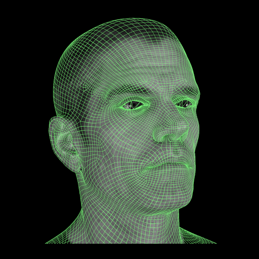
The rasterization operation takes as inputs a tensor of vertex positions and a tensor of vertex index triplets that specify the triangles. Vertex positions are specified in clip space, i.e., after modelview and projection transformations. Performing these transformations is left as the user's responsibility. In clip space, the view frustum is a cube in homogeneous coordinates where x/w, y/w, z/w are all between -1 and +1.

The output of the rasterization operation is a 4-channel float32 image with tuple (u, v, z/w, triangle_id) in each pixel. Values u and v are the barycentric coordinates within a triangle: the first vertex in the vertex index triplet obtains (u, v) = (1, 0), the second vertex (u, v) = (0, 1) and the third vertex (u, v) = (0, 0). Normalized depth value z/w is used later by the antialiasing operation to infer occlusion relations between triangles, and it does not propagate gradients to the vertex position input. Field triangle_id is the triangle index, offset by one. Pixels where no triangle was rasterized will receive a zero in all channels.

Rasterization is point-sampled, i.e., the geometry is not smoothed, blurred, or made partially transparent in any way, in contrast to some previous differentiable rasterizers. The contents of a pixel always represent a single surface point that is on the closest surface visible along the ray through the pixel center.

Point-sampled coverage does not produce vertex position gradients related to occlusion and visibility effects. This is because the motion of vertices does not change the coverage in a continuous way — a triangle is either rasterized into a pixel or not. In nvdiffrast, the occlusion/visibility related gradients are generated in the antialiasing operation that typically occurs towards the end of the rendering pipeline.

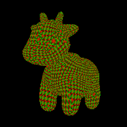
[..., 0:2] = barycentrics (u, v)

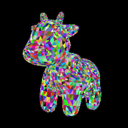
[..., 3] = triangle_id

The images above illustrate the output of the rasterizer. The left image shows the contents of channels 0 and 1, i.e., the barycentric coordinates, rendered as red and green, respectively. The right image shows channel 3, i.e., the triangle ID, using a random color per triangle. Spot model was created and released into public domain by Keenan Crane.

Interpolation

Depending on the shading and lighting models, a mesh typically specifies a number of attributes at its vertices. These can include, e.g., texture coordinates, vertex normals, reflection vectors, and material parameters. The purpose of the interpolation operation is to transfer these attributes specified at vertices to image space. In the hardware graphics pipeline, this happens automatically between vertex and pixel shaders. The interpolation operation in nvdiffrast supports an arbitrary number of attributes.

Concretely, the interpolation operation takes as inputs the buffer produced by the rasterizer and a buffer specifying the vertex attributes. The output is an image-size buffer with as many channels as there are attributes. Pixels where no triangle was rendered will contain all zeros in the output.

Texture coordinates (s, t)

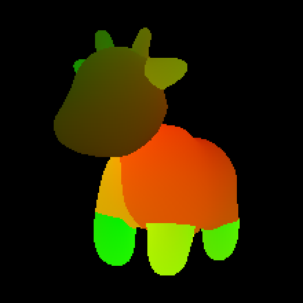
Above is an example of interpolated texture coordinates visualized in red and green channels. This image was created using the output of the rasterizer from the previous step, and an attribute buffer containing the texture coordinates.

Texturing

Texture sampling is a fundamental operation in hardware graphics pipelines, and the same is true in nvdiffrast. The basic principle is simple: given a per-pixel texture coordinate vector, fetch a value from a texture and place it in the output. In nvdiffrast, the textures may have an arbitrary number of channels, which is useful in case you want to learn, say, an abstract field that acts as an input to a neural network further down the pipeline.

When sampling a texture, it is typically desirable to use some form of filtering. Most previous differentiable rasterizers support at most bilinear filtering, where sampling at a texture coordinate between texel centers will interpolate the value linearly from the four nearest texels. While this works fine when viewing the texture up close, it yields badly aliased results when the texture is viewed from a distance. To avoid this, the texture needs to be prefiltered prior to sampling it, removing the frequencies that are too high compared to how densely it is being sampled.

Nvdiffrast supports prefiltered texture sampling based on mipmapping. The required mipmap levels can be generated internally in the texturing operation, so that the user only needs to specify the highest-resolution (base level) texture. Currently the highest-quality filtering mode is isotropic trilinear filtering. The lack of anisotropic filtering means that a texture viewed at a steep angle will not alias in any direction, but it may appear blurry across the non-squished direction.

In addition to standard 2D textures, the texture sampling operation also supports cube maps. Cube maps are addressed using 3D texture coordinates, and the transitions between cube map faces are properly filtered so there will be no visible seams. Cube maps support trilinear filtering similar to 2D textures. There is no explicit support for 1D textures but they can be simulated efficiently with 1×n textures. All the filtering, mipmapping etc. work with such textures just as they would with true 1D textures. For now there is no support for 3D volume textures.

Texture of Spot

Output of the texture sampling operation

Background replaced with white

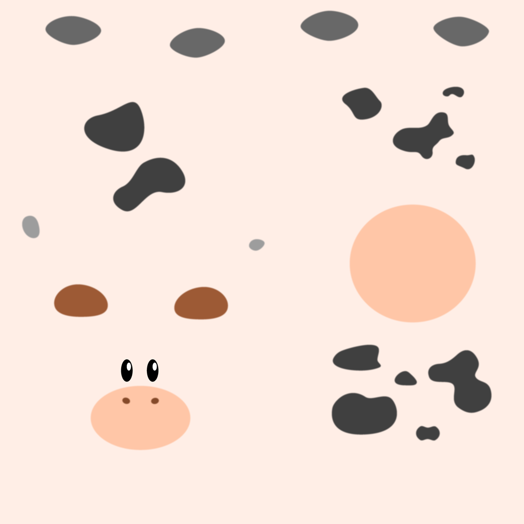
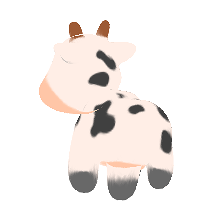
The middle image above shows the result of texture sampling using the interpolated texture coordinates from the previous step. Why is the background pink? The texture coordinates (s, t) read as zero at those pixels, but that is a perfectly valid point to sample the texture. It happens that Spot's texture (left) has pink color at its (0, 0) corner, and therefore all pixels in the background obtain that color as a result of the texture sampling operation. On the right, we have replaced the color of the empty pixels with a white color. Here's one way to do this in PyTorch:

img_right = torch.where(rast_out[..., 3:] > 0, img_left, torch.tensor(1.0).cuda())

where rast_out is the output of the rasterization operation. We simply test if the triangle_id field, i.e., channel 3 of the rasterizer output, is greater than zero, indicating that a triangle was rendered in that pixel. If so, we take the color from the textured image, and otherwise we take constant 1.0.

Antialiasing

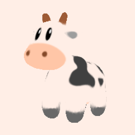
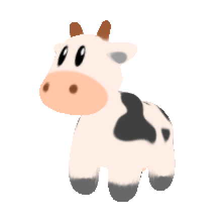
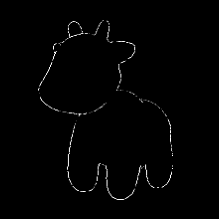
The last of the four primitive operations in nvdiffrast is antialiasing. Based on the geometry input (vertex positions and triangles), it will smooth out discontinuties at silhouette edges in a given image. The smoothing is based on a local approximation of coverage — an approximate integral over a pixel is calculated based on the exact location of relevant edges and the point-sampled colors at pixel centers.

In this context, a silhouette is any edge that connects to just one triangle, or connects two triangles so that one folds behind the other. Specifically, this includes both silhouettes against the background and silhouettes against another surface, unlike some previous methods (DIB-R) that only support the former kind.

It is worth discussing why we might want to go through this trouble to improve the image a tiny bit. If we're attempting to, say, match a real-world photograph, a slightly smoother edge probably won't match the captured image much better than a jagged one. However, that is not the point of the antialiasing operation — the real goal is to obtain gradients w.r.t. vertex positions related to occlusion, visibility, and coverage.

Remember that everything up to this point in the rendering pipeline is point-sampled. In particular, the coverage, i.e., which triangle is rasterized to which pixel, changes discontinuously in the rasterization operation.

This is the reason why previous differentiable rasterizers apply nonstandard image synthesis model with blur and transparency: Something has to make coverage continuous w.r.t. vertex positions if we wish to optimize vertex positions, camera position, etc., based on an image-space loss. In nvdiffrast, we do everything point-sampled so that we know that every pixel corresponds to a single, well-defined surface point. This lets us perform arbitrary shading computations without worrying about things like accidentally blurring texture coordinates across silhouettes, or having attributes mysteriously tend towards background color when getting close to the edge of the object. Only towards the end of the pipeline, the antialiasing operation ensures that the motion of vertex positions results in continuous change on silhouettes.

The antialiasing operation supports any number of channels in the image to be antialiased. Thus, if your rendering pipeline produces an abstract representation that is fed to a neural network for further processing, that is not a problem.

Antialiased image

Closeup, before AA

Closeup, after AA

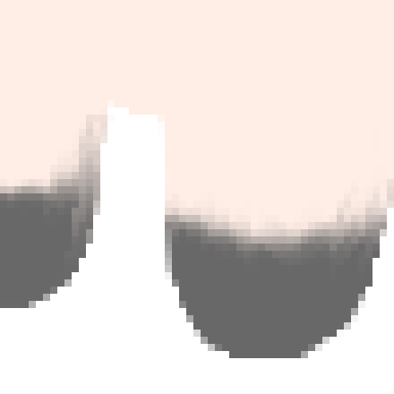
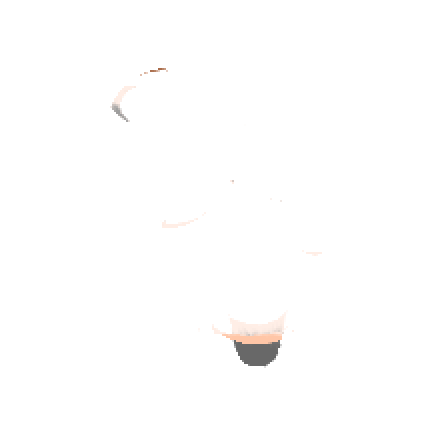
The left image above shows the result image from the last step, after performing antialiasing. The effect is quite small — some boundary pixels become less jagged, as shown in the closeups.

Notably, not all boundary pixels are antialiased as revealed by the left-side image below. This is because the accuracy of the antialiasing operation in nvdiffrast depends on the rendered size of triangles: Because we store knowledge of just one surface point per pixel, antialiasing is possible only when the triangle that contains the actual geometric silhouette edge is visible in the image. The example image is rendered in very low resolution and the triangles are tiny compared to pixels. Thus, triangles get easily lost between the pixels.

This results in incomplete-looking antialiasing, and the gradients provided by antialiasing become noisier when edge triangles are missed. Therefore it is advisable to render images in resolutions where the triangles are large enough to show up in the image at least most of the time.

Pixels touched by antialiasing, original resolution

Rendered in 4×4 higher resolution and downsampled

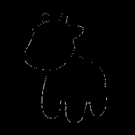
The left image above shows which pixels were modified by the antialiasing operation in this example. On the right, we performed the rendering in 4×4 higher resolution and downsampled the final images back to the original size. This yields more accurate position gradients related to the silhouettes, so if you suspect your position gradients are too noisy, you may want to try simply increasing the resolution in which rasterization and antialiasing is done.

For purposes of shape optimization, the sparse-looking situation on the left would probably be perfectly fine. The gradients are still going to point in the right direction even if they are somewhat sparse, and you will need to use some sort of shape regularization anyway, which will greatly increase tolerance to noisy shape gradients.

Beyond the basics

Rendering images is easy with nvdiffrast, but there are a few practical things that you will need to take into account. The topics in this section explain the operation and usage of nvdiffrast in more detail, and hopefully help you avoid any potential misunderstandings and pitfalls.

Coordinate systems

Nvdiffrast follows OpenGL's coordinate systems and other conventions. This is partially because we support OpenGL to accelerate the rasterization operation, but mostly so that there is a single standard to follow.

• In OpenGL convention, the perspective projection matrix (as implemented in, e.g., utils.projection() in our samples and glFrustum() in OpenGL) treats the view-space z as increasing towards the viewer. However, after multiplication by perspective projection matrix, the homogeneous clip-space coordinate z/w increases away from the viewer. Hence, a larger depth value in the rasterizer output tensor also corresponds to a surface further away from the viewer.
• The memory order of image data in OpenGL, and consequently in nvdiffrast, is bottom-up. This means that row 0 of a tensor containing an image is the bottom row of the texture/image, which is the opposite of the more common scanline order. If you want to keep your image data in the conventional top-down order in your code, but have it logically the right way up inside nvdiffrast, you will need to flip the images vertically when crossing the boundary.
• For 2D textures, the coordinate origin (s, t) = (0, 0) is at the bottom left corner with s increasing to the right and t increasing to the top. When specifying the faces of a cube map texture, the orientation varies between the faces, but nvdiffrast follows the OpenGL convention here as well.

As a word of advice, it is best to stay on top of coordinate systems and orientations used in your program. When something appears to be the wrong way around, it is much better to identify and fix the root cause than to randomly flip coordinates, images, buffers, and matrices until the immediate problem goes away.

Geometry and minibatches: Range mode vs Instanced mode

As mentioned earlier, all operations in nvdiffrast support the minibatch axis efficiently. Related to this, we support two ways for representing the geometry: range mode and instanced mode. If you want to render a different mesh in each minibatch index, you need to use the range mode. However, if you are rendering the same mesh, but with potentially different viewpoints, vertex positions, attributes, textures, etc., in each minibatch index, the instanced mode will be much more convenient.

In range mode, you specify triangle index triplets as a 2D tensor of shape [num_triangles, 3], and vertex positions as a 2D tensor of shape [num_vertices, 4]. In addition to these, the rasterization operation requires an additional 2D range tensor of shape [minibatch_size, 2] where each row specifies a start index and count into the triangle tensor. As a result, the rasterizer will render the triangles in the specified ranges into each minibatch index of the output tensor. If you have multiple meshes, you should place all of them into the vertex and triangle tensors, and then choose which mesh to rasterize into each minibatch index via the contents of the range tensor. The attribute tensor in interpolation operation is handled in the same way as positions, and it has to be of shape [num_vertices, num_attributes] in range mode.

In instanced mode, the topology of the mesh will be shared for each minibatch index. The triangle tensor is still a 2D tensor with shape [num_triangles, 3], but the vertex positions are specified using a 3D tensor of shape [minibatch_size, num_vertices, 4]. With a 3D vertex position tensor, the rasterizer will not require the range tensor input, but will take the minibatch size from the first dimension of the vertex position tensor. The same triangles are rendered to each minibatch index, but with vertex positions taken from the corresponding slice of the vertex position tensor. In this mode, the attribute tensor in interpolation has to be a 3D tensor similar to position tensor, i.e., of shape [minibatch_size, num_vertices, num_attributes]. However, you can provide an attribute tensor with minibatch size of 1, and it will be broadcast across the minibatch.

Image-space derivatives

We skirted around a pretty fundamental question in the description of the texturing operation above. In order to determine the proper amount of prefiltering for sampling a texture, we need to know how densely it is being sampled. But how can we know the sampling density when each pixel knows of a just a single surface point?

The solution is to track the image-space derivatives of all things leading up to the texture sampling operation. These are not the same thing as the gradients used in the backward pass, even though they both involve differentiation! Consider the barycentrics (u, v) produced by the rasterization operation. They change by some amount when moving horizontally or vertically in the image plane. If we denote the image-space coordinates as (X, Y), the image-space derivatives of the barycentrics would be ∂u/∂X, ∂u/∂Y, ∂v/∂X, and ∂v/∂Y. We can organize these into a 2×2 Jacobian matrix that describes the local relationship between (u, v) and (X, Y). This matrix is generally different at every pixel. For the purpose of image-space derivatives, the units of X and Y are pixels. Hence, ∂u/∂X is the local approximation of how much u changes when moving a distance of one pixel in the horizontal direction, and so on.

Once we know how the barycentrics change w.r.t. pixel position, the interpolation operation can use this to determine how the attributes change w.r.t. pixel position. When attributes are used as texture coordinates, we can therefore tell how the texture sampling position (in texture space) changes when moving around within the pixel (up to a local, linear approximation, that is). This texture footprint tells us the scale on which the texture should be prefiltered. In more practical terms, it tells us which mipmap level(s) to use when sampling the texture.

In nvdiffrast, the rasterization operation outputs the image-space derivatives of the barycentrics in an auxiliary 4-channel output tensor, ordered (∂u/∂X, ∂u/∂Y, ∂v/∂X, ∂v/∂Y) from channel 0 to 3. The interpolation operation can take this auxiliary tensor as input and compute image-space derivatives of any set of attributes being interpolated. Finally, the texture sampling operation can use the image-space derivatives of the texture coordinates to determine the amount of prefiltering.

There is nothing magic about these image-space derivatives. They are tensors like the, e.g., the texture coordinates themselves, they propagate gradients backwards, and so on. For example, if you want to artificially blur or sharpen the texture when sampling it, you can simply multiply the tensor carrying the image-space derivatives of the texture coordinates ∂{s, t}/∂{X, Y} by a scalar value before feeding it into the texture sampling operation. This scales the texture footprints and thus adjusts the amount of prefiltering. If your loss function prefers a different level of sharpness, this multiplier will receive a nonzero gradient. Update: Since version 0.2.1, the texture sampling operation also supports a separate mip level bias input that would be better suited for this particular task, but the gist is the same nonetheless.

One might wonder if it would have been easier to determine the texture footprints simply from the texture coordinates in adjacent pixels, and skip all this derivative rubbish? In easy cases the answer is yes, but silhouettes, occlusions, and discontinuous texture parameterizations would make this approach rather unreliable in practice. Computing the image-space derivatives analytically keeps everything point-like, local, and well-behaved.

It should be noted that computing gradients related to image-space derivatives is somewhat involved and requires additional computation. At the same time, they are often not crucial for the convergence of the training/optimization. Because of this, the primitive operations in nvdiffrast offer options to disable the calculation of these gradients. We're talking about things like ∂Loss/∂(∂{u, v}/∂{X, Y}) that may look second-order-ish, but they're not.

Mipmaps and texture dimensions

Prefiltered texture sampling modes require mipmaps, i.e., downsampled versions, of the texture. The texture sampling operation can construct these internally, or you can provide your own mipmap stack, but there are limits to texture dimensions that need to be considered.

When mipmaps are constructed internally, each mipmap level is constructed by averaging 2×2 pixel patches of the preceding level (or of the texture itself for the first mipmap level). The size of the buffer to be averaged therefore has to be divisible by 2 in both directions. There is one exception: side length of 1 is valid, and it will remain as 1 in the downsampling operation.

For example, a 32×32 texture will produce the following mipmap stack:

And a 32×8 texture, with both sides powers of two but not equal, will result in:

For texture sizes like this, everything will work automatically and mipmaps are constructed down to 1×1 pixel size. Therefore, if you wish to use prefiltered texture sampling, you should scale your textures to power-of-two dimensions that do not, however, need to be equal.

How about texture atlases? You may have an object whose texture is composed of multiple individual patches, or a collection of textured meshes with a unique texture for each. Say we have a texture atlas composed of five 32×32 sub-images, i.e., a total size of 160×32 pixels. Now we cannot compute mipmap levels all the way down to 1×1 size, because there is a 5×1 mipmap in the way that cannot be downsampled (because 5 is not even):

Scaling the atlas to, say, 256×32 pixels would feel silly because the dimensions of the sub-images are perfectly fine, and downsampling the different sub-images together — which would happen after the 5×1 resolution — would not make sense anyway. For this reason, the texture sampling operation allows the user to specify the maximum number of mipmap levels to be constructed and used. In this case, setting max_mip_level=5 would stop at the 5×1 mipmap and prevent the error.

It is a deliberate design choice that nvdiffrast doesn't just stop automatically at a mipmap size it cannot downsample, but requires the user to specify a limit when the texture dimensions are not powers of two. The goal is to avoid bugs where prefiltered texture sampling mysteriously doesn't work due to an oddly sized texture. It would be confusing if a 256×256 texture gave beautifully prefiltered texture samples, a 255×255 texture suddenly had no prefiltering at all, and a 254×254 texture did just a bit of prefiltering (one level) but not more.

If you compute your own mipmaps, their sizes must follow the scheme described above. There is no need to specify mipmaps all the way to 1×1 resolution, but the stack can end at any point and it will work equivalently to an internally constructed mipmap stack with a max_mip_level limit. Importantly, the gradients of user-provided mipmaps are not propagated automatically to the base texture — naturally so, because nvdiffrast knows nothing about the relation between them. Instead, the tensors that specify the mip levels in a user-provided mipmap stack will receive gradients of their own.

Rasterizing with CUDA vs OpenGL (New!)

Since version 0.3.0, nvdiffrast on PyTorch supports executing the rasterization operation using either CUDA or OpenGL. Earlier versions and the Tensorflow bindings support OpenGL only.

When rasterization is executed on OpenGL, we use the GPU's graphics pipeline to determine which triangles land on which pixels. GPUs have amazingly efficient hardware for doing this — it is their original raison d'être — and thus it makes sense to exploit it. Unfortunately, some computing environments haven't been designed with this in mind, and it can be difficult to get OpenGL to work correctly and interoperate with CUDA cleanly. On Windows, compatibility is generally good because the GPU drivers required to run CUDA also include OpenGL support. Linux is more complicated, as various drivers can be installed separately and there isn't a standardized way to acquire access to the hardware graphics pipeline.

Rasterizing in CUDA pretty much reverses these considerations. Compatibility is obviously not an issue on any CUDA-enabled platform. On the other hand, implementing the rasterization process correctly and efficiently on a massively data-parallel programming model is non-trivial. The CUDA rasterizer in nvdiffrast follows the approach described in research paper High-Performance Software Rasterization on GPUs by Laine and Karras, HPG 2011. Our code is based on the paper's publicly released CUDA kernels, with considerable modifications to support current hardware architectures and to match nvdiffrast's needs.

The CUDA rasterizer does not support output resolutions greater than 2048×2048, and both dimensions must be multiples of 8. In addition, the number of triangles that can be rendered in one batch is limited to around 16 million. Subpixel precision is limited to 4 bits and depth peeling is less accurate than with OpenGL. Memory consumption depends on many factors.

It is difficult to predict which rasterizer offers better performance. For complex meshes and high resolutions OpenGL will most likely outperform the CUDA rasterizer, although it has certain overheads that the CUDA rasterizer does not have. For simple meshes and low resolutions the CUDA rasterizer may be faster, but it has its own overheads, too. Measuring the performance on actual data, on the target platform, and in the context of the entire program is the only way to know for sure.

To run rasterization in CUDA, create a RasterizeCudaContext and supply it to the rasterize() operation. For OpenGL, use a RasterizeGLContext instead. Easy!

Running on multiple GPUs

Nvdiffrast supports computation on multiple GPUs in both PyTorch and TensorFlow. As is the convention in PyTorch, the operations are always executed on the device on which the input tensors reside. All GPU input tensors must reside on the same device, and the output tensors will unsurprisingly end up on that same device. In addition, the rasterization operation requires that its context was created for the correct device. In TensorFlow, the rasterizer context is automatically created on the device of the rasterization operation when it is executed for the first time.

The remainder of this section applies only to OpenGL rasterizer contexts. CUDA rasterizer contexts require no special considerations besides making sure they're on the correct device.

On Windows, nvdiffrast implements OpenGL device selection in a way that can be done only once per process — after one context is created, all future ones will end up on the same GPU. Hence you cannot expect to run the rasterization operation on multiple GPUs within the same process using an OpenGL context. Trying to do so will either cause a crash or incur a significant performance penalty. However, with PyTorch it is common to distribute computation across GPUs by launching a separate process for each GPU, so this is not a huge concern. Note that any OpenGL context created within the same process, even for something like a GUI window, will prevent changing the device later. Therefore, if you want to run the rasterization operation on other than the default GPU, be sure to create its OpenGL context before initializing any other OpenGL-powered libraries.

On Linux everything just works, and you can create OpenGL rasterizer contexts on multiple devices within the same process.

Note on torch.nn.DataParallel

PyTorch offers torch.nn.DataParallel wrapper class for splitting the execution of a minibatch across multiple threads. Unfortunately, this class is fundamentally incompatible with OpenGL-dependent operations, as it spawns a new set of threads at each call (as of PyTorch 1.9.0, at least). Using previously created OpenGL contexts in these new threads, even if taking care to not use the same context in multiple threads, causes them to be migrated around and this has resulted in ever-growing GPU memory usage and abysmal GPU utilization. Therefore, we advise against using torch.nn.DataParallel for rasterization operations that depend on the OpenGL contexts.

Notably, torch.nn.DistributedDataParallel spawns subprocesses that are much more persistent. The subprocesses must create their own OpenGL contexts as part of initialization, and as such they do not suffer from this problem.

GitHub issue #23, especially this comment, contains further analysis and suggestions for workarounds.

Rendering multiple depth layers

Sometimes there is a need to render scenes with partially transparent surfaces. In this case, it is not sufficient to find only the surfaces that are closest to the camera, as you may also need to know what lies behind them. For this purpose, nvdiffrast supports depth peeling that lets you extract multiple closest surfaces for each pixel.

With depth peeling, we start by rasterizing the closest surfaces as usual. We then perform a second rasterization pass with the same geometry, but this time we cull all previously rendered surface points at each pixel, effectively extracting the second-closest depth layer. This can be repeated as many times as desired, so that we can extract as many depth layers as we like. See the images below for example results of depth peeling with each depth layer shaded and antialiased.

First depth layer

Second depth layer

Third depth layer

The API for depth peeling is based on DepthPeeler object that acts as a context manager, and its rasterize_next_layer method. The first call to rasterize_next_layer is equivalent to calling the traditional rasterize function, and subsequent calls report further depth layers. The arguments for rasterization are specified when instantiating the DepthPeeler object. Concretely, your code might look something like this:

with nvdiffrast.torch.DepthPeeler(glctx, pos, tri, resolution) as peeler:
  for i in range(num_layers):
    rast, rast_db = peeler.rasterize_next_layer()
    (process or store the results)

There is no performance penalty compared to the basic rasterization op if you end up extracting only the first depth layer. In other words, the code above with num_layers=1 runs exactly as fast as calling rasterize once.

Depth peeling is only supported in the PyTorch version of nvdiffrast. For implementation reasons, depth peeling reserves the rasterizer context so that other rasterization operations cannot be performed while the peeling is ongoing, i.e., inside the with block. Hence you cannot start a nested depth peeling operation or call rasterize inside the with block unless you use a different context.

For the sake of completeness, let us note the following small caveat: Depth peeling relies on depth values to distinguish surface points from each other. Therefore, culling "previously rendered surface points" actually means culling all surface points at the same or closer depth as those rendered into the pixel in previous passes. This matters only if you have multiple layers of geometry at matching depths — if your geometry consists of, say, nothing but two exactly overlapping triangles, you will see one of them in the first pass but never see the other one in subsequent passes, as it's at the exact depth that is already considered done.

Differences between PyTorch and TensorFlow

Nvdiffrast can be used from PyTorch and from TensorFlow 1.x; the latter may change to TensorFlow 2.x if there is demand. These frameworks operate somewhat differently and that is reflected in the respective APIs. Simplifying a bit, in TensorFlow 1.x you construct a persistent graph out of persistent nodes, and run many batches of data through it. In PyTorch, there is no persistent graph or nodes, but a new, ephemeral graph is constructed for each batch of data and destroyed immediately afterwards. Therefore, there is also no persistent state for the operations. There is the torch.nn.Module abstraction for festooning operations with persistent state, but we do not use it.

As a consequence, things that would be part of persistent state of an nvdiffrast operation in TensorFlow must be stored by the user in PyTorch, and supplied to the operations as needed. In practice, this is a very small difference and amounts to just a couple of lines of code in most cases.

As an example, consider the OpenGL context used by the rasterization operation. In order to use hardware-accelerated rendering, an OpenGL context must be created and switched into before issuing OpenGL commands internally. Creating the context is an expensive operation, so we don't want to create and destroy one at every call of the rasterization operation. In TensorFlow, the rasterization operation creates a context when it is executed for the first time, and stashes it away in its persistent state to be reused later. In PyTorch, the user has to create the context using a separate function call, and supply it as a parameter to the rasterization operation.

Similarly, if you have a constant texture and want to use prefiltered texture sampling modes, the mipmap stack only needs to be computed once. In TensorFlow, you can specify that the texture is constant, in which case the texture sampling operation only computes the mipmap stack on the first execution and stores it internally. In PyTorch, you can compute the mipmap stack once using a separate function call, and supply it to the texture sampling operation every time. If you don't do that, the operation will compute the mipmap stack internally and discard it afterwards. This is exactly what you want if your texture changes at every iteration, and it's not wrong even if the texture is constant, just a bit inefficient.

Finally, the same holds for a thing called the topology hash that the antialiasing operation uses for identifying potential silhouette edges. Its contents depend only on the triangle tensor, not the vertex positions, so if the topology is constant, this auxiliary structure needs to be constructed only once. As before, in TensorFlow this is handled internally, whereas in PyTorch a separate function is provided for off-line construction.

Manual OpenGL contexts in PyTorch

First, please note that handling OpenGL contexts manually is a very small optimization. It almost certainly won't be relevant unless you've already profiled and optimized your code with gusto, and you're on a mission to extract every last bit of performance possible.

In TensorFlow, the only option is to let nvdiffrast handle the OpenGL context management internally. This is because TensorFlow utilizes multiple CPU threads under the hood, and the active OpenGL context is a thread-local resource.

PyTorch isn't as unpredictable, and stays in the same CPU thread by default (although things like torch.utils.data.DataLoader do invoke additional CPU threads). As such, nvdiffrast lets the user choose between handling OpenGL context switching in automatic or manual mode. The default is automatic mode where the rasterization operation always sets/releases the context at the beginning/end of each execution, like we do in TensorFlow. This ensures that the rasterizer will always use the context that you supply, and the context won't remain active so nobody else can mess with it.

In manual mode, the user assumes the responsibility of setting and releasing the OpenGL context. Most of the time, if you don't have any other libraries that would be using OpenGL, you can just set the context once after having created it and keep it set until the program exits. However, keep in mind that the active OpenGL context is a thread-local resource, so it needs to be set in the same CPU thread as it will be used, and it cannot be set simultaneously in multiple CPU threads.

Samples

Nvdiffrast comes with a set of samples that were crafted to support the research paper. Each sample is available in both PyTorch and TensorFlow versions. Details such as command-line parameters, logging format, etc., may not be identical between the versions, and generally the PyTorch versions should be considered definitive. The command-line examples below are for the PyTorch versions.

All PyTorch samples support selecting between CUDA and OpenGL rasterizer contexts. The default is to do rasterization in CUDA, and switching to OpenGL is done by specifying command-line option --opengl.

Enabling interactive display using the --display-interval parameter is likely to fail on Linux when using OpenGL rasterization. This is because the interactive display window is shown using OpenGL, and on Linux this conflicts with the internal OpenGL rasterization in nvdiffrast. Using a CUDA context should work, assuming that OpenGL is correctly installed in the system (for displaying the window). Our Dockerfile is set up to support headless rendering only, and thus cannot show an interactive result window.

triangle.py

This is a minimal sample that renders a triangle and saves the resulting image into a file (tri.png) in the current directory. Running this should be the first step to verify that you have everything set up correctly. Rendering is done using the rasterization and interpolation operations, so getting the correct output image means that both OpenGL (if specified on command line) and CUDA are working as intended under the hood.

This is the only sample where you must specify either --cuda or --opengl on command line. Other samples default to CUDA rasterization and provide only the --opengl option.

Example command lines:

python triangle.py --cuda
python triangle.py --opengl

The expected output image

cube.py

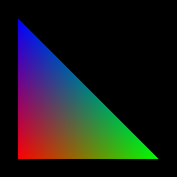
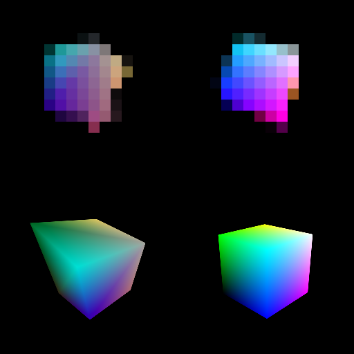
In this sample, we optimize the vertex positions and colors of a cube mesh, starting from a semi-randomly initialized state. The optimization is based on image-space loss in extremely low resolutions such as 4×4, 8×8, or 16×16 pixels. The goal of this sample is to examine the rate of geometrical convergence when the triangles are only a few pixels in size. It serves to illustrate that the antialiasing operation, despite being approximative, yields good enough position gradients even in 4×4 resolution to guide the optimization to the goal.

Example command line:

python cube.py --resolution 16 --display-interval 10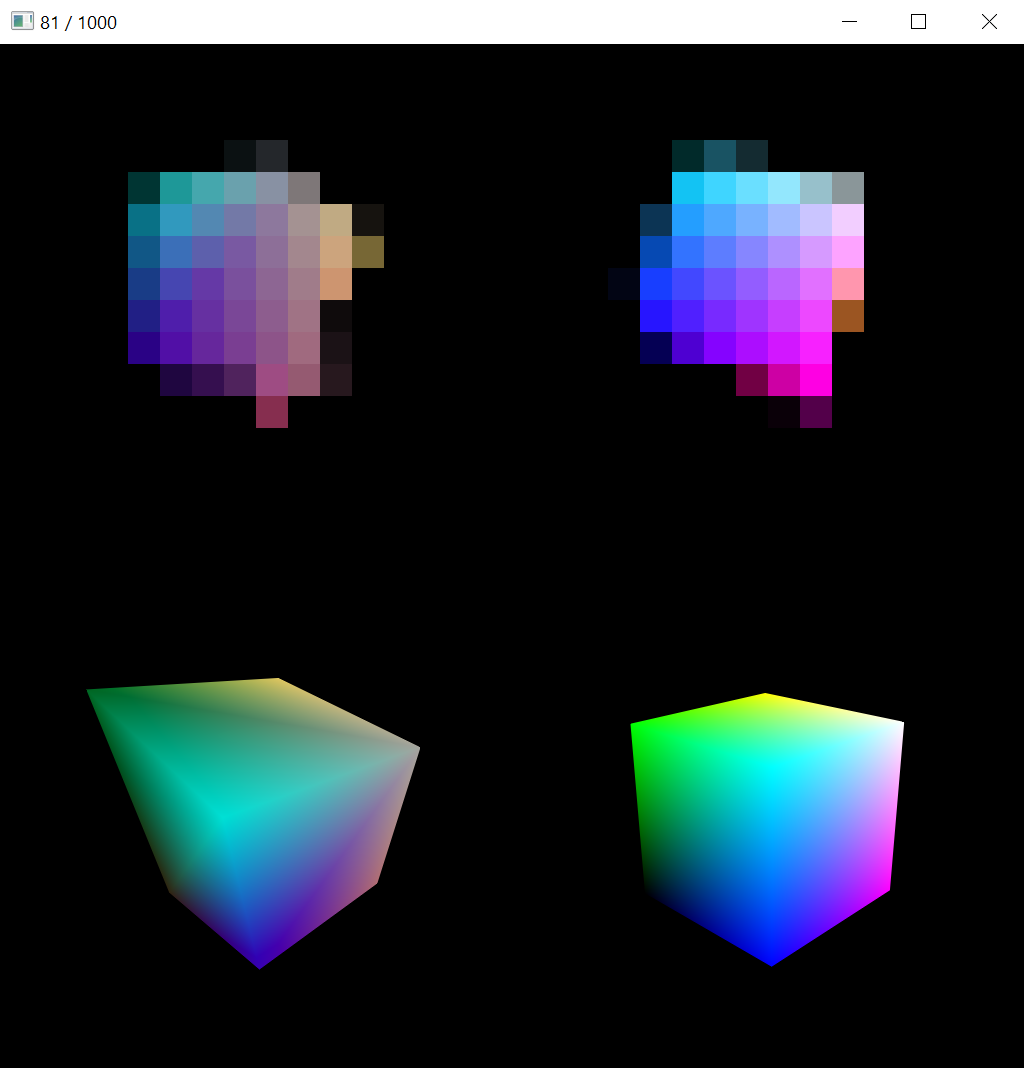

Interactive view of cube.py

Rendering pipeline

The image above shows a live view of the sample. Top row shows the low-resolution rendered image and reference image that the image-space loss is calculated from. Bottom row shows the current mesh (and colors) and reference mesh in high resolution so that convergence can be seen more easily visually.

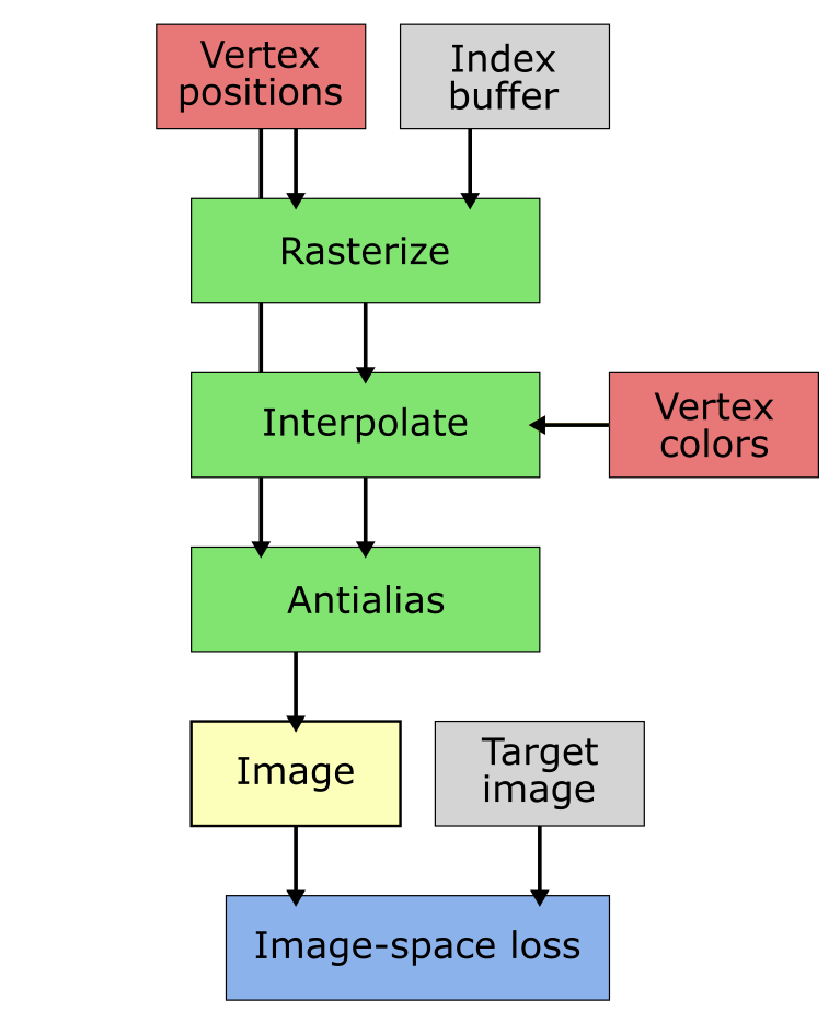
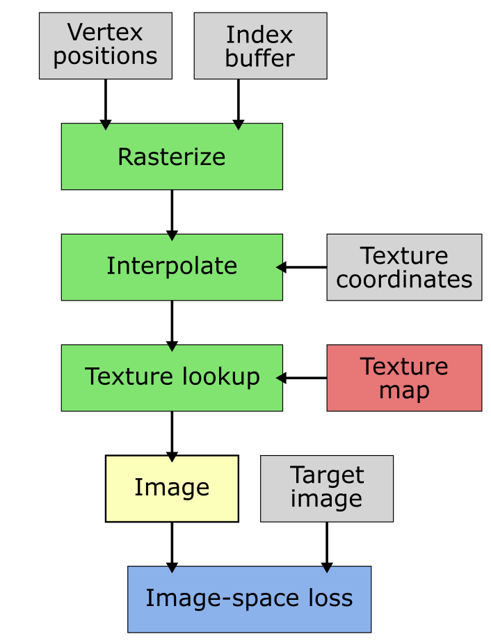
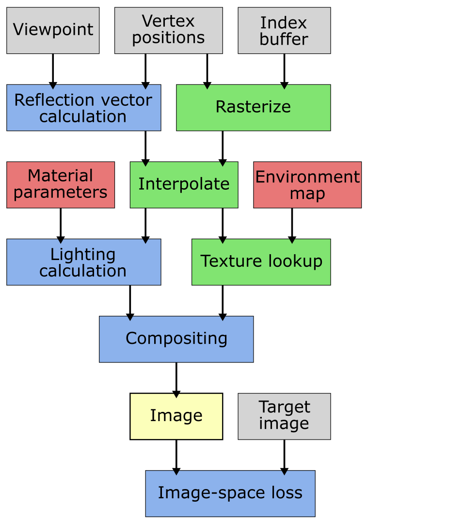
In the pipeline diagram, green boxes indicate nvdiffrast operations, whereas blue boxes are other computation. Red boxes are the learned tensors and gray are non-learned tensors or other data.

earth.py

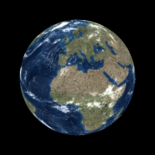
The goal of this sample is to compare texture convergence with and without prefiltered texture sampling. The texture is learned based on image-space loss against high-quality reference renderings in random orientations and at random distances. When prefiltering is disabled, the texture is not learned properly because of spotty gradient updates caused by aliasing. This shows as a much worse PSNR for the texture, compared to learning with prefiltering enabled. See the paper for further discussion.

Example command lines:

Interactive view of earth.py, prefiltering disabled

Rendering pipeline

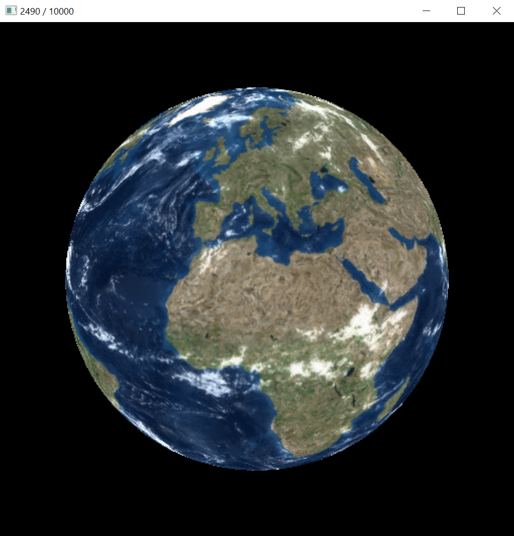
The interactive view shows the current texture mapped onto the mesh, with or without prefiltered texture sampling as specified via the command-line parameter. In this sample, no antialiasing is performed because we are not learning vertex positions and hence need no gradients related to them.

envphong.py

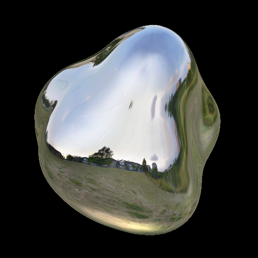
In this sample, a more complex shading model is used compared to the vertex colors or plain texture in the previous ones. Here, we learn a reflected environment map and parameters of a Phong BRDF model given a known mesh. The optimization is based on image-space loss against reference renderings in random orientations. The shading model of mirror reflection plus a Phong BRDF is not physically sensible, but it works as a reasonably simple strawman that would not be possible to implement with previous differentiable rasterizers that bundle rasterization, shading, lighting, and texturing together. The sample also illustrates the use of cube mapping for representing a learned texture in a spherical domain.

Example command line:

python envphong.py --display-interval 10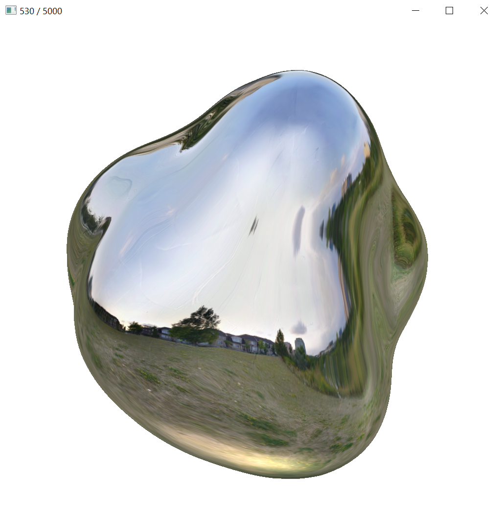

Interactive view of envphong.py

Rendering pipeline

In the interactive view, we see the rendering with the current environment map and Phong BRDF parameters, both gradually improving during the optimization.

pose.py

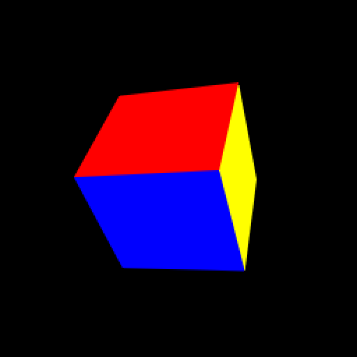
Pose fitting based on an image-space loss is a classical task in differentiable rendering. In this sample, we solve a pose optimization problem with a simple cube with differently colored sides. We detail the optimization method in the paper, but in brief, it combines gradient-free greedy optimization in an initialization phase and gradient-based optimization in a fine-tuning phase.

Example command line:

python pose.py --display-interval 10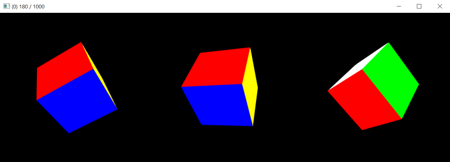

Interactive view of pose.py

The interactive view shows, from left to right: target pose, best found pose, and current pose. When viewed live, the two stages of optimization are clearly visible. In the first phase, the best pose updates intermittently when a better initialization is found. In the second phase, the solution converges smoothly to the target via gradient-based optimization.

PyTorch API reference

Licenses

Copyright © 2020–2023, NVIDIA Corporation. All rights reserved.

This work is made available under the Nvidia Source Code License.

For business inquiries, please visit our website and submit the form: NVIDIA Research Licensing

We do not currently accept outside contributions in the form of pull requests.

Environment map stored as part of samples/data/envphong.npz is derived from a Wave Engine sample material originally shared under MIT License. Mesh and texture stored as part of samples/data/earth.npz are derived from 3D Earth Photorealistic 2K model originally made available under TurboSquid 3D Model License.

Citation

@article{Laine2020diffrast,
  title   = {Modular Primitives for High-Performance Differentiable Rendering},
  author  = {Samuli Laine and Janne Hellsten and Tero Karras and Yeongho Seol and Jaakko Lehtinen and Timo Aila},
  journal = {ACM Transactions on Graphics},
  year    = {2020},
  volume  = {39},
  number  = {6}
}

Acknowledgements

We thank David Luebke, Simon Yuen, Jaewoo Seo, Tero Kuosmanen, Sanja Fidler, Wenzheng Chen, Jacob Munkberg, Jon Hasselgren, and Onni Kosomaa for discussions, test data, support with compute infrastructure, testing, reviewing, and suggestions for features and improvements.