Sol-Engine · Research blog
Interactive Coding Worlds with Real-time Streaming Diffusion Render
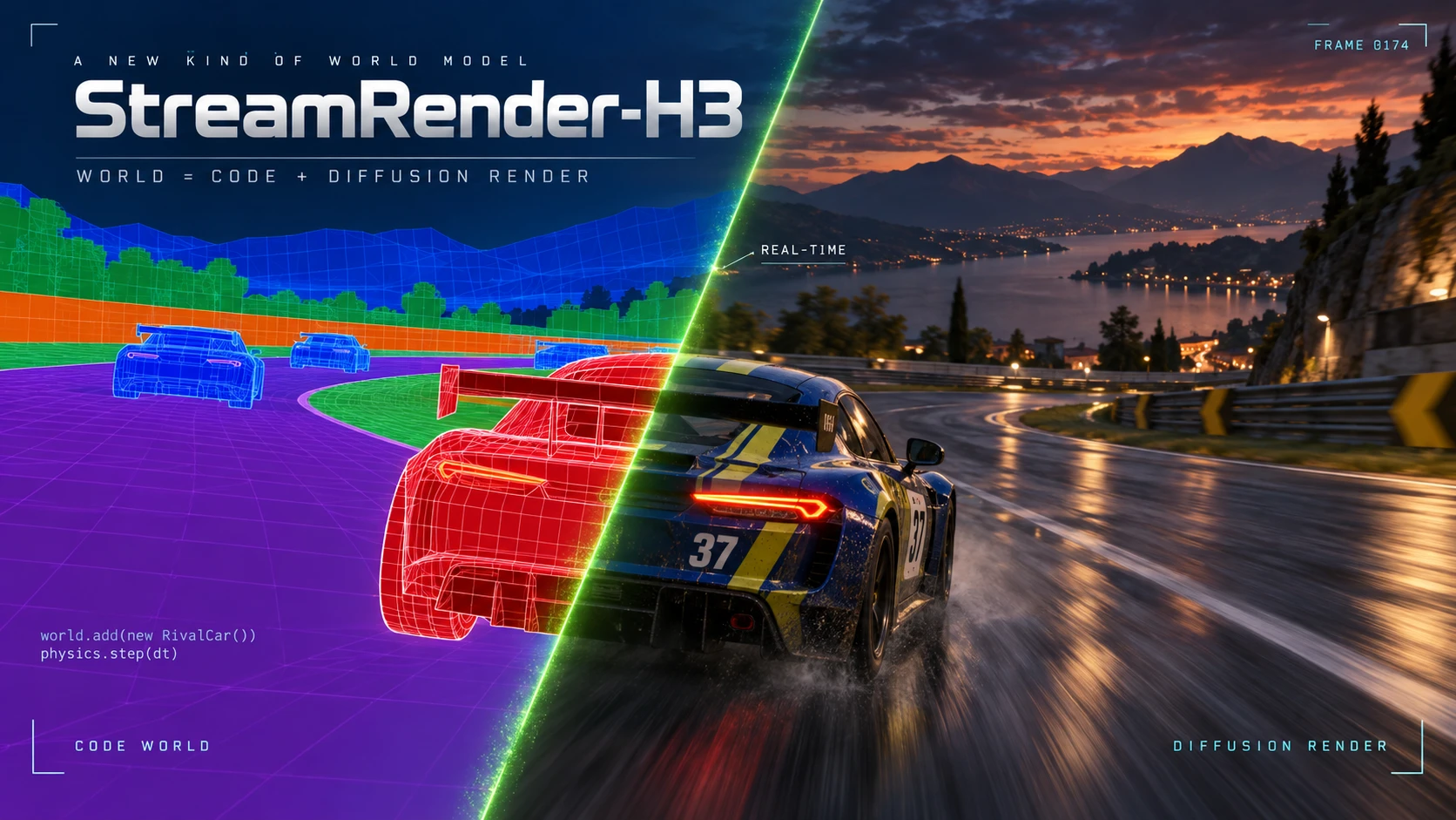
Code drives the world, video models generate the visuals. A code game engine keeps the world state, and a two-step streaming video model renders it as the player drives.
Why Separate World Logic from Visual Generation
An interactive world must determine how player actions change its state and how those changes appear on screen. World logic governs maps, physics, rules, and object states. Visual generation determines appearance, materials, lighting, and style. Game engines already separate these responsibilities, and video models offer a new way to produce the visuals.
World logic requires explicit, controllable state. Road positions should be queryable, collisions should follow executable rules, and revisiting a location should return the same map. Code directly represents and maintains this information, allowing developers to modify rules, debug behavior, and reproduce interactions. Video models can use reference conditions to give the same scene structure and motion different appearances.
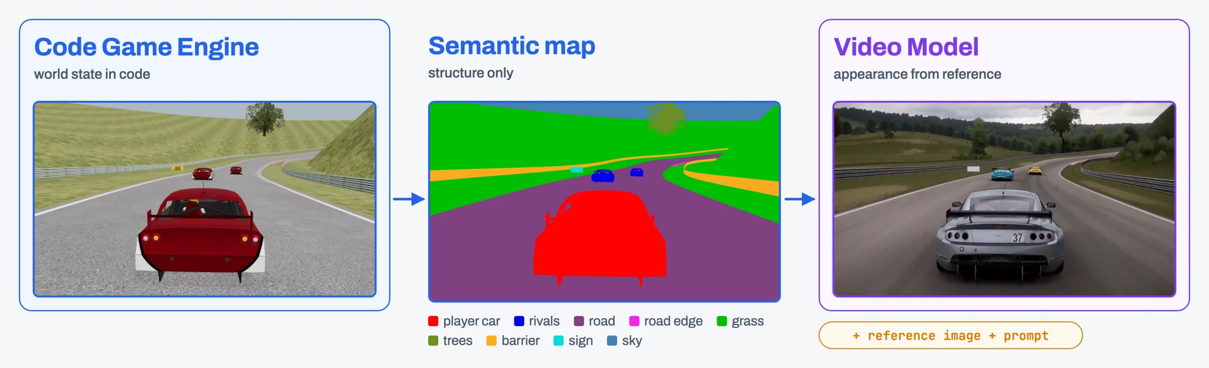
StreamRender-H3 separates these responsibilities between a Code Game Engine and a Streaming Diffusion Render. The engine maintains world state and responds to player input, while the video model continuously generates the visuals. An intermediate state representation connects the two. This preserves control over the world while enabling flexible, high-fidelity visuals without relying on a traditional 3D pipeline for final rendering.
Overall Architecture: Code Game Engine × Streaming Diffusion Render
2.1Code Game Engine: Maps, Physics, and Interaction Feedback
The Code Game Engine maintains every part of the world that code can state exactly. Throughout this post we use a racing game as the running demo. It serves only as an example, and nothing in the design is specific to racing. In the racing demo, the engine is a browser game written in three.js. In general, the engine keeps three kinds of information.
Maps. A map describes the geometry and layout of the scene, the objects placed in it, and the class to which each object belongs. In the racing demo, the map holds the track with its edges and barriers and the scenery along the route. Because the map lives in code, any part of it can be queried at any time, and returning to a location shows exactly the same scene.
Physics and rules. Physics and rules determine how objects move and interact, such as how a body responds to the player's input, what happens in a collision, and how non-player characters behave. They advance with a fixed time step, so the same sequence of inputs always produces the same trajectory, which makes behavior easy to debug and replay. Scripted agents can also play the game on their own, which lets us record reproducible sessions without a human player. In the racing scenario, every car in the recorded training sessions is driven by an AI driver.
Interaction feedback. At every step, the engine reads the player's input, advances the world, and reports where every object is and where the camera points. It then draws the current state from the camera's viewpoint. This drawing does not need to look good. It only needs to convey the structure of the scene precisely, in the form described in Section 2.2, because producing the image that the player sees is the task of the video model.
2.2Intermediate State Representations: Connecting World State and Visual Generation
The engine and the video model need a common representation. This representation must carry everything that the world logic decides, such as where objects are, what shapes they have, how they move, and where the camera points. At the same time, it should carry nothing about how objects look, so that appearance is left entirely to the video model. Depth maps, edge maps, and low-fidelity renders of the game itself all satisfy these requirements to some degree.
We currently use semantic maps, in which every pixel is painted with a flat color that identifies the class of the object it shows, without lighting, texture, or shading. A semantic map contains the layout of the scene, the outline and position of every object, their motion, and the camera path, which are exactly the quantities that the world logic determines. Because it contains no appearance, the same play session can be rendered in different styles. A semantic map is also inexpensive to produce, since any engine that can draw its scene with one flat color per class can drive the renderer, and this keeps the interface open to other games and engines. In the racing demo, the semantic map distinguishes 13 classes, namely road, road edge, terrain, grass, vegetation, rock, barrier, building, grandstand, billboard, sky, the player's car, and rival cars. These classes and their colors are fixed and shared between training and deployment.
The video model is built on MiniMax-H3 Ref2VA, a model that generates video and audio from a prompt together with reference images and reference videos. The semantic stream enters it as a reference video. Each of its latent frames is aligned with the output latent frame at the same time step, so the semantic video determines the structure of every generated frame.
2.3A Real-Time Interaction Loop from Player Input to Video Feedback
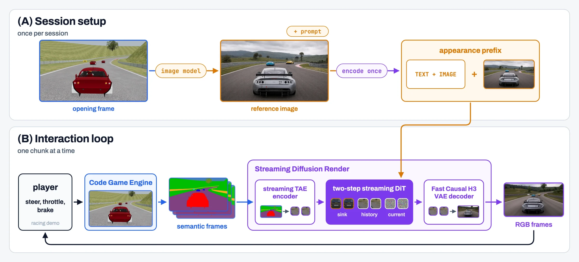
Interactive play differs from offline video generation in two ways. The video cannot be produced in advance, because its content depends on inputs that the player has not given yet. Each input must also appear on screen quickly enough for the player to react to it. StreamRender-H3 therefore runs as a loop in which the engine and the renderer work on the same stream at the same time, and the player sees the result while the next part is still being generated.
A session consists of two phases. Setup happens once at the beginning. The engine draws the opening frame of the scene, an image generation model turns this frame into a photorealistic reference image, and the reference image and the prompt are encoded once and kept for the entire session (Section 3.1.1). The interaction loop then runs without pause, and each pass through it consists of five steps.
- The player gives an input through the keyboard or a controller. In the racing demo, this input steers, accelerates, or brakes the player's car.
- The engine applies the input at its next physics step and advances the world.
- The engine draws one semantic frame for every video frame and streams these frames to the renderer.
- The renderer collects the semantic frames of one chunk, which covers a fraction of a second of video. It generates the chunk in a few denoising steps, two in the racing demo, conditioned on the appearance of the session and on its own recent output, and decodes the result into RGB frames.
- The frames are displayed, and the player reacts to them in the next pass of the loop.
The loop runs in real time when each chunk is ready before the previous one has finished playing. The video then keeps pace with play, and each input shows up as soon as the chunk that contains its effect has been generated. The engine and the renderer share only the semantic frame stream and the appearance conditions of the session, so either side can be replaced independently. A different game, for example, only needs to produce semantic frames in the same format. Sections 3.2 and 3.3 describe how decoding and generation fit within the playback time of each chunk.
Key Technologies
3.1Streaming Diffusion Render
The streaming diffusion render turns the semantic stream of the engine into photorealistic video. This section describes how it is conditioned and trained. Section 3.1.1 explains how a reference image and a prompt fix the look of the world. The video is produced by a diffusion generator that is trained in three stages. Section 3.1.2 explains how each chunk stays consistent with the stream before it and covers the two pre-training stages, teacher forcing and Resampling Forcing. Section 3.1.3 covers the last stage, DMD, which lets the generator produce each chunk in two steps for real-time play.
3.1.1Appearance Control Driven by Reference Images and Prompts
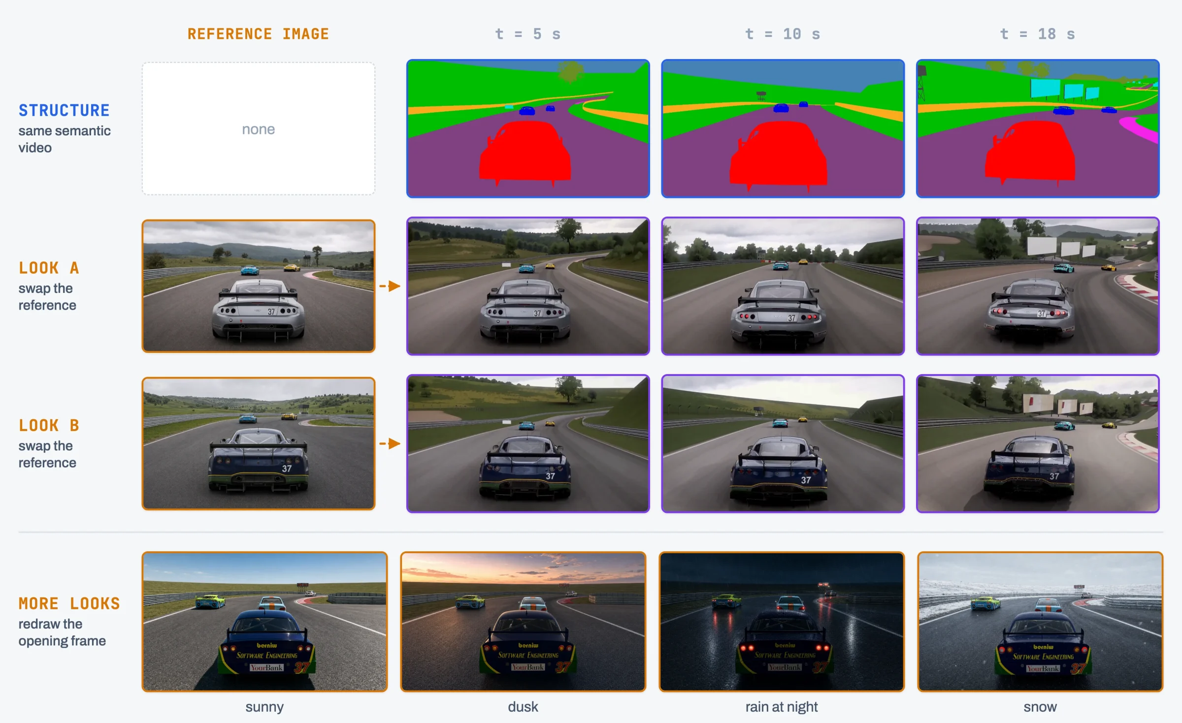
A semantic map tells the renderer where everything is, but not what it looks like. In the racing demo, for example, the same road class could become dry asphalt at noon or a wet street at night, and the same vehicle class could become any car in any color. The renderer therefore needs a second source of information that fixes the look of the world. This information must also stay the same for the whole session, so that objects keep their appearance as the stream goes on. A prompt alone is too coarse for this purpose, because a few sentences cannot pin down a particular material, color scheme, or lighting. We therefore give the renderer two inputs at the start of each session, a reference image that shows the intended look and a prompt that explains how the inputs relate to each other.
Reference image. An image generation model redraws the opening frame of the game as a photorealistic picture. The redrawn picture keeps the composition of the frame, including the camera view, the layout of the scene, and the position of every object, and it chooses the materials, the colors and markings of objects, the weather, the lighting, and the overall style. Since the picture is aligned with the first semantic frame, each object in it corresponds to a region of a known class, so the renderer can tell which appearance belongs to which class. Changing the instruction given to the image model is enough to produce a different look for the same opening frame.
Prompt. The prompt follows the structured template of MiniMax-H3. It defines the subjects of the scene and states which input controls each of their properties. The look of each subject comes from the reference image, whereas its outline, position, and motion, as well as the camera path, come from the semantic video. In the racing demo, the prompt defines three subjects, namely the player's car, the rival cars, and the track with its surroundings. The prompt also states which object class each color of the semantic video represents, and it describes the rendering style, the lighting, and the sound.
Replacing the reference image and the prompt changes the look of the same game, while the engine and the semantic stream remain unchanged.
Training data in the racing scenario. For the racing demo, the renderer learns this division of labor from 10,000 paired clips of racing gameplay, each about 15 seconds long. The clips are cut from about 5,100 recorded races on 39 tracks, which include road circuits, dirt tracks, and ovals. Every car in these races is driven by an AI driver, each race has between zero and fifteen rival cars, and the camera follows the player's car from behind. For every clip, the engine records its normal render and the semantic video at 1344×768 and 24 frames per second. Each clip then receives three conditions and one target.
- Reference image. An image editing model (GPT-Image-2.5) redraws the first frame of the normal render as a screenshot of a modern photorealistic racing game. It keeps the camera, the road course, every car at its position and size, and the colors of the rival cars, and the player's car keeps the livery colors and the number it has in the game. Everything else is redesigned in rich detail. Fine detail, such as spectators in a grandstand, is added only to regions that already hold that kind of object, and no car is added. The clips are assigned ten lighting looks in turn, so that each look covers 1,000 clips. The looks are clear midday sun, early morning sun, golden hour, sunset, blue hour, overcast sky, broken clouds, summer haze, morning mist, and storm clouds with a shaft of sunlight.
- Prompt. An LLM agent (Claude Opus 5.5) prepares both the reference image and the prompts. It watches the normal render and the semantic video, sends the first frame to the image model, and writes one prompt for each segment of the target in the template described above. Besides the subjects, the style, and the sound, each prompt narrates the events of its segment in time order with timestamps, such as when the player's car enters a bend or passes a rival.
- Target video. The native MiniMax-H3 Ref2VA model generates the photorealistic target from the reference image, the semantic video, and the prompt with 25 denoising steps. The native model can generate a whole 15-second clip at once, but we found that after about five seconds the generated video no longer follows the semantic video and the reference image closely. Each 15-second clip is therefore produced as three consecutive segments of about five seconds, and each segment starts from the last frame of the previous one.
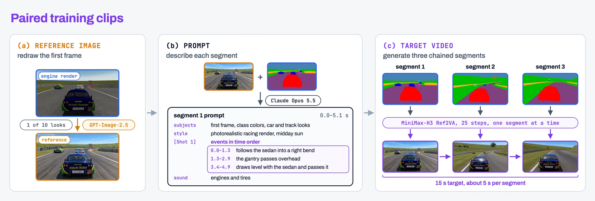
The pre-training of Section 3.1.2 uses these targets. The DMD stage of Section 3.1.3 learns from critics rather than from targets, so it is trained on longer recordings that need no target. In the racing scenario, these are 5,000 drives of 60 seconds from the same recorded races, each with its semantic video, a reference image, and a prompt.
3.1.2Historical Context and Temporal Consistency
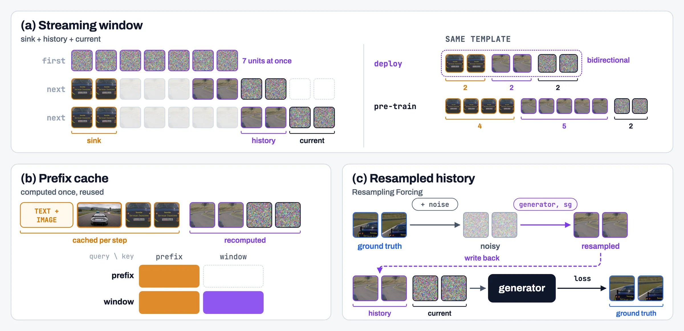
The renderer generates the video chunk by chunk, and every chunk must remain consistent with what came before it. Following the streaming design of LynnReal-Omni, we denoise each chunk in a single window together with two kinds of context. The first is the sink, the opening part of the stream, which stays in every window for the whole session. It anchors the identity of the scene and its objects, in the same spirit as the attention sink of StreamingLLM and the frame sink of LongLive. The second is the recent history, the part generated immediately before the current chunk, which carries motion across chunk boundaries. Attention inside the window is bidirectional. Every window after the first is mapped onto the same position template, so a window late in the stream appears to the generator exactly like an early one.
In the racing demo, the deployed generator produces two scheduling units per chunk, each holding one or two latent frames, and it keeps two units of sink and two units of recent history. The first window of a stream generates seven units at once, which provides later windows with a full context from the start. During pre-training, the generator uses a wider window with four units of sink and five units of recent history.
Prefix cache. The text and image conditioning, the reference image, and the sink no longer change after the first continuation. We therefore split each window into a fixed prefix and a moving part, and we let the prefix attend only to itself while the moving part attends to the entire window. At inference, the keys and values of the prefix are computed once for each denoising step and reused for every later chunk, so only the recent history and the current chunk are recomputed (Section 3.3). The DMD stage of Section 3.1.3 trains with the same attention mask and recomputes the prefix with the current weights, so the generator is trained on exactly the computation it performs at inference. During pre-training, attention is dense within each window.
Streaming training. The generator is fine-tuned from MiniMax-H3 Ref2VA in three stages. Teacher forcing and then Resampling Forcing pre-train it as an ordinary multi-step diffusion model, and DMD then trains it to generate each chunk in two steps for real-time play (Section 3.1.3). In the racing demo, pre-training uses the paired racing clips of Section 3.1.1. Every stage trains on windows with the same layout of sink, recent history, and current chunk as at inference, and the stages differ in where the history comes from. Teacher forcing samples one window from each clip and takes its history from the ground truth. Resampling Forcing and DMD instead run along streams. Every training clip forms a stream of consecutive windows. Each training step processes one window of every stream, and the output of that window is written back as history for the next window, which a later step processes. Resampling Forcing writes back resampled versions of the ground truth as described below, and DMD writes back the chunks that the generator produces itself (Section 3.1.3).
Resampling Forcing. After teacher forcing, the generator has seen only ground-truth history. At inference, however, its context is its own imperfect output, and its errors then accumulate along the stream. We close this gap with the resampling operation of Resampling Forcing. Resampling Forcing trains a causal autoregressive video model end to end and uses self-resampling to expose it to its own errors on the history frames. Our generator keeps bidirectional attention inside each window, so we borrow only the resampling itself and apply it to the history of each window. For each stream, a noise level is drawn from a shifted logit-normal distribution. At every window, the ground-truth chunk is noised to this level and resampled by the generator itself without gradient, and it is this resampled chunk rather than the ground truth that is written back as history. The current chunk is trained against the ground truth while being conditioned on the resampled history, so the generator learns to continue from context that contains its own errors.
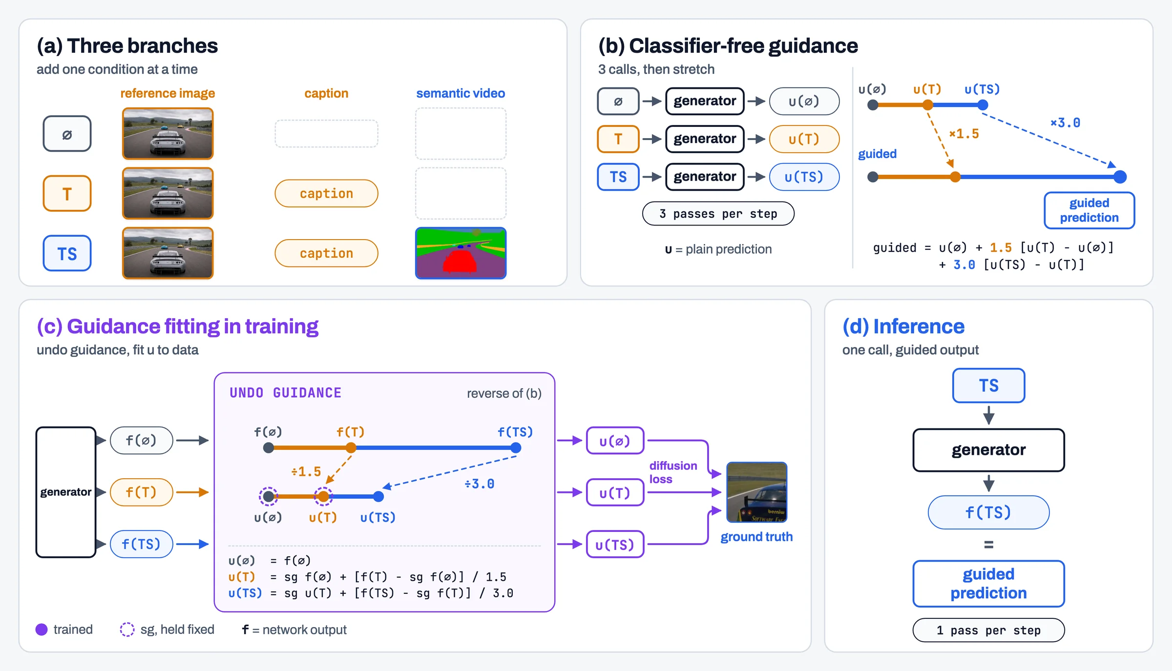
Guidance fitted into the generator. The released MiniMax-H3 checkpoint is guidance-distilled, so it samples with a single forward pass per denoising step. Following the semantic video closely, however, requires guidance on the structure condition as well, and classifier-free guidance over the caption and the semantic video would take three forward passes per step. LynnReal-Omni avoids this cost by training guidance into the model. It combines the conditional prediction of the model with a stop-gradient caption-free prediction and fits the combination to the data, so that at convergence the conditional prediction alone equals the guided prediction. LynnReal-Omni fits a single guidance step on the caption. We extend this approach to structure control with a chain of three branches. The branch ∅ receives neither the caption nor the semantic video, the branch T adds the caption, and the branch TS adds the semantic video, while the reference image is present in every branch. Classifier-free guidance along this chain starts from the plain conditional predictions u(∅), u(T), and u(TS). It stretches the caption step from u(∅) to u(T) by 1.5 and the structure step from u(T) to u(TS) by 3.0, which is the setting of the racing demo. Guidance fitting runs this chain backwards. We treat the raw outputs f(∅), f(T), and f(TS) of the network as guided predictions and undo the guidance by shrinking each step by its scale, which gives u(∅) = f(∅), u(T) = f(∅) + [f(T) − f(∅)] / 1.5, and u(TS) = u(T) + [f(TS) − f(T)] / 3.0. The start of each step is held fixed with a stop gradient, so that u(T) = (2 f(T) + sg f(∅)) / 3 and u(TS) = (f(TS) + sg f(T) + sg f(∅)) / 3, and every u is trained against the data with the ordinary diffusion loss. Once each u matches the plain conditional prediction, applying the guidance to u returns f, so a single call of f(TS) gives the guided prediction. Placing the strongest guidance on the step that adds the semantic video keeps the layout, the objects, and the camera of the generated video consistent with the state of the engine. The generator learns guidance fitting together with Resampling Forcing in the same pre-training run, so each of its denoising steps takes a single forward pass.
3.1.3Two-Step Distillation and Autoregressive Streaming Generation
Even with guidance fitted, the pre-trained generator is too slow for real-time play. In the racing demo, it samples each chunk with 16 denoising steps, whereas real-time play leaves only a fraction of a second to generate a chunk. We therefore continue training it with DMD, so that it generates each chunk in two steps while continuing its own stream.
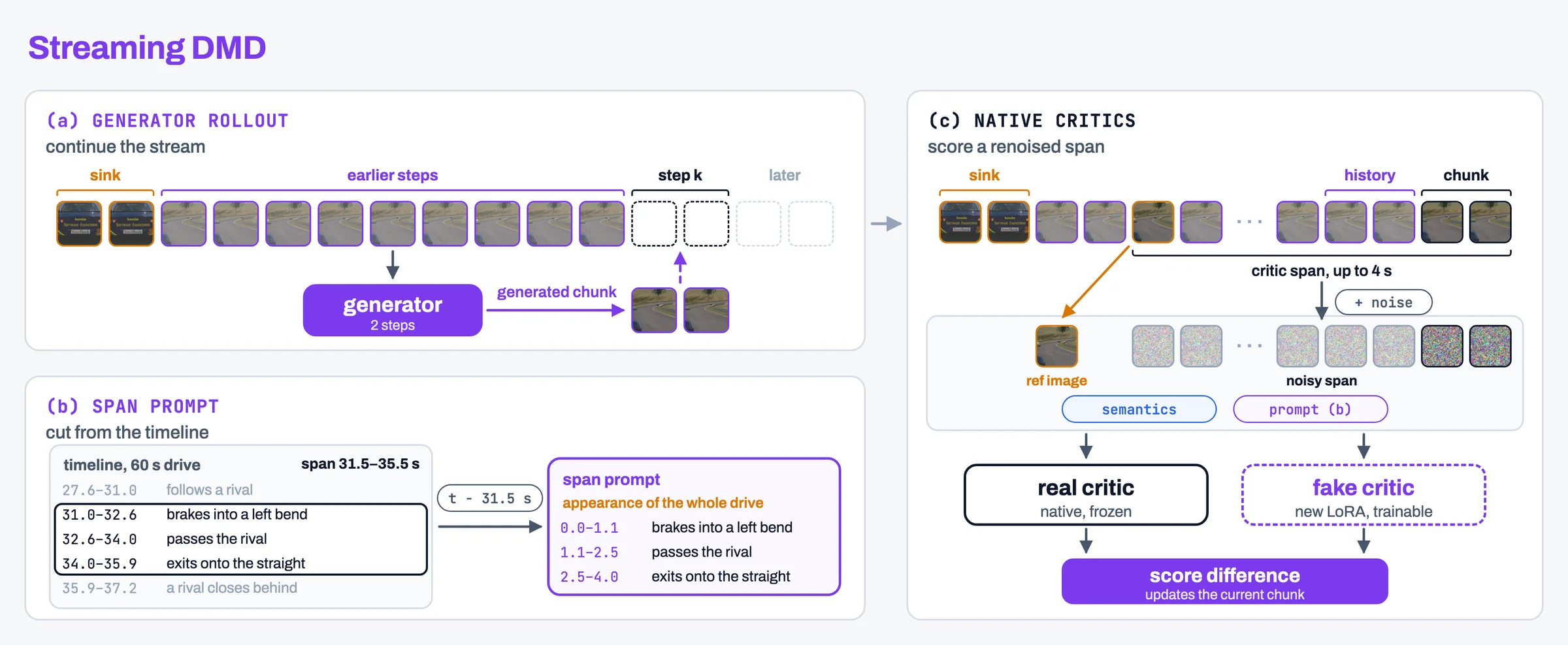
Two-step generation. In the racing demo, the generator produces each chunk in two denoising steps, first from pure noise to an intermediate noise level and then to a clean chunk, and it continues from its own output chunk after chunk with the window and prefix cache of Section 3.1.2. Its window of two sink units, two history units, and two current units is smaller than the one used in pre-training, which keeps each step inexpensive. It is trained along streams like Resampling Forcing, but without any ground truth. In the racing demo, each of its training streams covers the first 30 seconds of a 60-second drive (Section 3.1.1).
Streaming distribution matching distillation. We train the generator with distribution matching distillation (DMD, DMD2). A frozen real critic represents the distribution that the generator should reach, and a trainable fake critic tracks what the generator currently produces. The difference between their scores on a re-noised generated chunk tells the generator how to move toward the real critic. As in Self Forcing, the generator is trained on its own rollout rather than on ground truth. Following the streaming training of Section 3.1.2, each step generates the current window of every stream from the generator's own earlier output, computes the loss on that chunk only, and writes the generated chunk back, so that the next step continues the same stream. The history of later windows has therefore been generated by earlier versions of the generator, and no gradient flows into it. This follows the same idea as the streaming long tuning of LongLive, which extends the clip from the previous iteration and applies DMD only to the newly generated segment. Our streams, however, advance by one chunk per step rather than by several seconds.
Critics on a short span. Both critics are the native bidirectional MiniMax-H3 Ref2VA, and each scores a short continuous span of the rollout that ends at the current chunk. The frame of the rollout at the start of the span serves as the reference image, and the semantic video of the same span serves as the reference video. In the racing demo, a span holds up to 29 latent frames, about four seconds. The real critic is the released model itself, frozen and without an adapter. The released checkpoint is guidance-distilled, so a single forward pass gives its prediction. The fake critic starts from the same released weights with a fresh LoRA, which trains on the generated spans with the guidance fitting of Section 3.1.2 at scales 3.0 and 4.0, and it scores with its plain conditional prediction u(TS). DMD therefore moves the generator toward what the released model generates for each span. The fake critic learns on the whole span, whereas the generator is updated through its current chunk only.
Prompts cut from a timeline. Each critic sees a different few seconds of a long drive, so its prompt must describe exactly that span. A prompt that describes the drive only in general terms is not enough. We found that without the actions of the span described with timestamps, the model does not know where on the timeline the reference image belongs, and it sometimes even renders the semantic video in reverse. Describing the look of the player's car in the prompt also keeps its colors right. We therefore label every 60-second drive once with a timeline. In the racing demo, an agent running GPT-6.1 Sol watches the semantic video together with two tables sampled every quarter second, the speed, acceleration, and yaw rate of the player's car recorded by the engine, and the position and size of every car in the semantic video. It also sees the redrawn first frame and an earlier general prompt of the drive, from which it takes the look of the cars and the track. It writes the appearance of every car and of the track, which holds for the whole drive, phases of 2 to 10 seconds that describe the course, events of 0.3 to 2.5 seconds with absolute timestamps, and the state of the scene every half second. For each score span, the events that fall inside it are cut out and shifted to the clock of the span, and they are assembled with the appearance, the phases that overlap the span, and the states at its start and end into a prompt in the template of Section 3.1.1. The generator keeps its single prompt for the whole session, so the prefix cache of Section 3.1.2 still applies.
3.2Fast Causal H3 VAE: Self-Improving the Streaming Decoder with Agent Loops
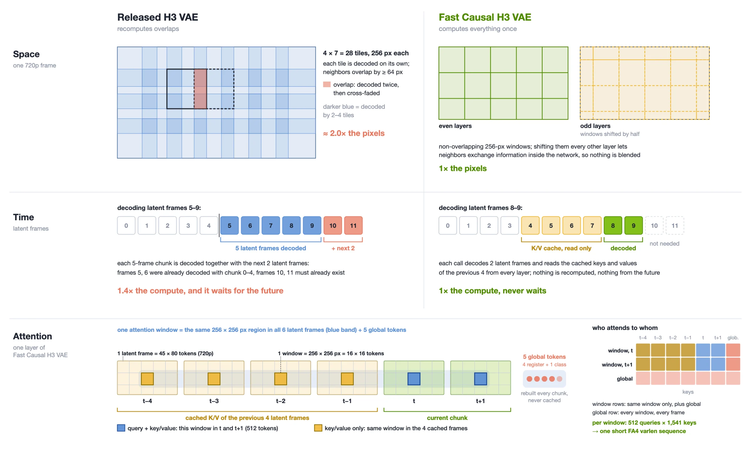
The streaming render produces latents, and a decoder turns them into the frames the player sees. In an interactive loop, each new latent frame must become pixels immediately, using only what has already been generated. The released H3 VAE decoder gives the best image quality, but it was built for offline video. It is a 36-layer Transformer with 2.42B parameters that relies on two kinds of overlap. Spatial tiling splits each frame into 256-pixel tiles that overlap by at least 64 pixels and blends the seams, so at 720p it decodes 28 tiles and computes every pixel about twice. Temporal chunking with overlap decodes five latent frames (17 video frames) at a time together with the next two latent frames, so it waits for latent frames that do not exist yet and computes each latent frame 1.4 times. It needs about 870 ms per five-latent-frame block at 720p. A tiny streaming decoder such as TAE runs in about 10 ms, but in our streaming runs it reached only 27 dB PSNR against the full VAE, kept 80% of its fine detail, and made grass, foliage, and road texture flicker from frame to frame.
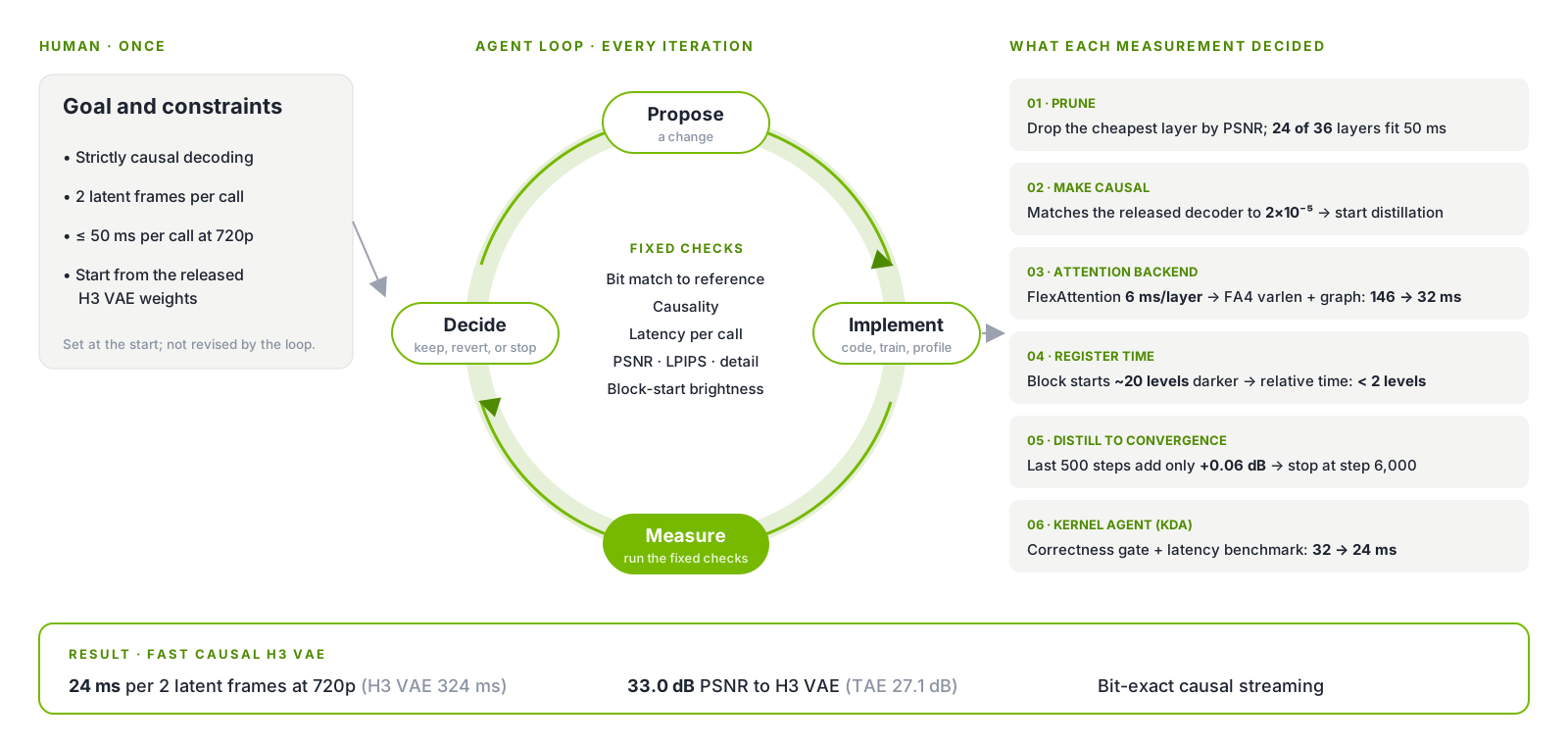
A decoder built by a loop. We did not design the new decoder by hand. We gave a coding agent (Claude Code) one goal and four constraints: decode strictly causally, take two latent frames per call, stay within 50 ms per call at 720p, and start from the released H3 VAE weights. From there the work ran as a loop. In each iteration the agent proposed a change, implemented it, and ran the same checks: a comparison against a reference decoder, a causality test that perturbs future latents, decode latency, and PSNR, LPIPS and fine detail against the H3 VAE. The numbers decided whether a change stayed, was reverted, or ended the search. About three hours after the goal was set, the causal decoder was running in the streaming pipeline, and distillation then continued to convergence. The paragraphs below follow the iterations in order.
Iteration 1: prune to fit the budget. The agent removed layers greedily without retraining. At each depth it dropped the layer whose removal cost the least reconstruction PSNR, and timed the result. 24 of the 36 layers fit the 50 ms budget at 720p and 540p, so the search stopped there. The kept layers are 0–17, 19–21, 31, 32, and 35 with their original weights, which brings the decoder to 1.62B parameters.
Iteration 2: make it causal, then check before training. The agent rewrote how the decoder sees time and space.
- Time. The DiT emits two or three latent frames per round, so the decoder works on chunks of two latent frames. Each chunk attends to its own two latent frames and to the cached keys and values of the previous four in every layer, about 0.7 s of video, and never to a later latent frame. Every call returns eight video frames. When a chunk contains the first latent frame of a native five-latent-frame block, that latent frame yields one video frame, exactly as in the released VAE, so the stream still produces 17 video frames per five latent frames. The context comes from cached past latent frames instead of recomputed future ones, so each latent frame is computed once.
- Space. Spatial tiling is removed. Attention runs within non-overlapping windows of 16×16 tokens, which cover the same 256 pixels as a tile, and every other layer shifts the windows by half a window so that neighboring windows exchange information inside the network. Every pixel is computed once and no seam blending is needed. Spatial positions are encoded relative to the window, as in the released tile decode.
Before any training, the rewritten decoder was run in a non-causal reference mode and compared with the released decoder. The two matched to within 2×10⁻⁵, so the rewrite itself added no error and distillation could start.
Iteration 3: measure where the time goes. Run naively in PyTorch, the model takes 146 ms per two latent frames at 720p, three times the budget. Profiling showed that matrix multiplications took only about 15 ms of this. The rest went to copying the cache and re-partitioning windows (36 ms), masked attention on a slow kernel (30 ms), and many small element-wise kernels (30 ms), including a cast of all weights from fp32 to bf16 on every call. Each measured cost became the next change, and none of the changes alters the computation:
- Linear-layer weights are stored in bf16 once, instead of being cast on every call. The residual stream stays in fp32, as in training.
- The key-value cache is kept per window in a preallocated ring buffer. Each new latent frame receives its rotary position once and is written into its slot in place, so the cache is never concatenated or re-partitioned.
- Partitioning tokens into windows and merging them back become single index gathers, fused by
torch.compilewith normalization and rotary embedding. - Attention backends were timed on the actual shape. FlexAttention with a block mask took 6 ms per layer, more than the whole budget across 24 layers, so window attention runs through FlashAttention-4's variable-length interface instead. Each window is one short sequence, about 512 queries against 1,541 keys, padding positions are left out of the packed arrays, and
seqused_khides cache slots that are still empty at stream start, so no mask is needed. - Every chunk has the same shapes, so the whole chunk is captured once as a CUDA graph and replayed, which removes kernel-launch overhead (37 ms → 32 ms).
Iteration 4: a failure the averages missed. The decoder carries four register tokens and one class token that attend to the whole frame. They are rebuilt for every chunk and never cached, so they cannot carry information backward from a later chunk. In the released decoder these tokens have no time position, and that is harmless there: each temporal chunk is decoded on its own with its frames numbered from 0, so attention between frame tokens and register tokens only ever sees the same few time positions. The causal decoder cannot renumber its frames, because cached keys must keep the positions they were computed with, so frame tokens take the absolute latent-frame index of the stream. The first version kept the register tokens without a time position, so their attention to frame tokens depended on absolute time. Training clips held ten latent frames, and from the eleventh latent frame on, the first video frame of every five-latent-frame block turned about 20 gray levels darker. The averaged metrics did not show this; it appeared when we watched the decoded stream. Giving the register tokens the time position of their chunk makes every attention score depend only on time differences, and the gap fell below two gray levels. Two checks came out of this iteration: block-start brightness measured frame by frame, and decoding the same latent frames from different stream clocks. The output is now identical whether the clock starts at 0, 100, or 1000.
Iteration 5: distill to convergence. The teacher is the full H3 VAE decode of the same latents. The student decodes chunk by chunk with the same code used in deployment, on clips of three five-latent-frame blocks (51 video frames, 384×384 crops), so it sees block starts both with an empty cache and with a full one. The loss combines L1, LPIPS (weight 1.0), a frame-difference term (weight 1.0, tripled across latent boundaries), and an edge term (weight 0.1). Training used eight GPUs and AdamW at a learning rate of 2×10⁻⁵, decayed on a cosine schedule to 10⁻⁶ over the last 3,500 steps. Training stopped at step 6,000, when the last 500 steps had raised PSNR on the evaluation cases by only 0.06 dB. As a check on causality, changing any future latent frame leaves every earlier output frame bit-for-bit unchanged.
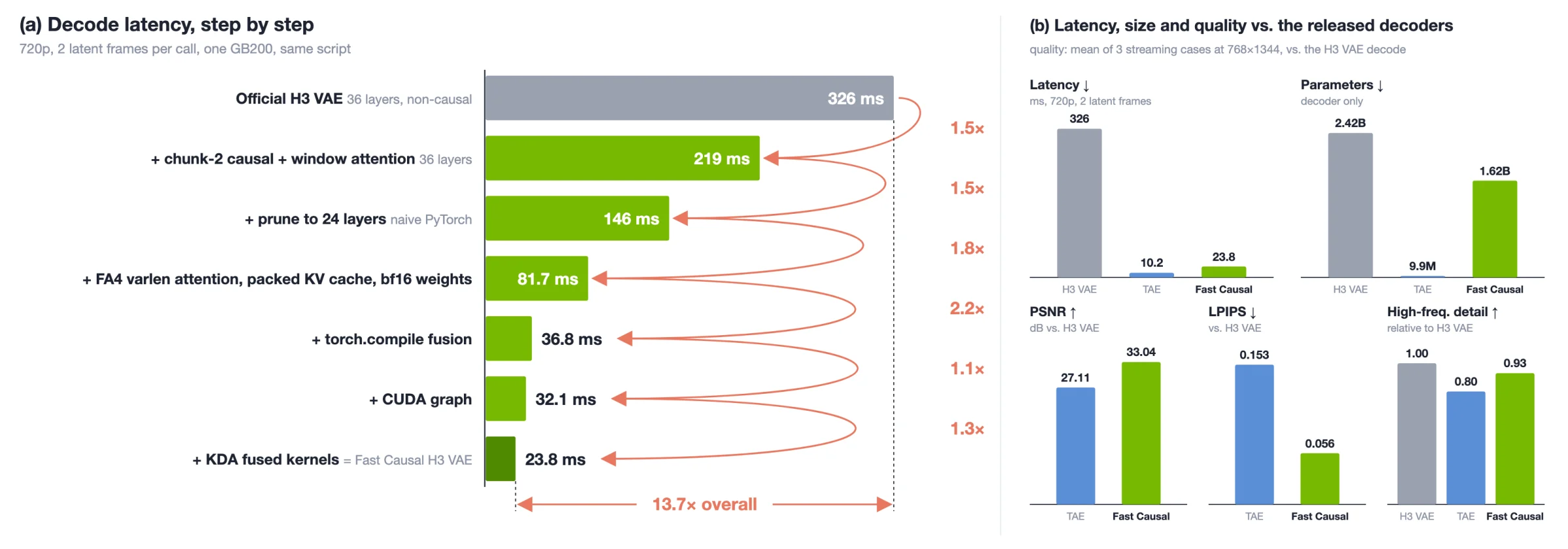
Iteration 6: a second loop for the kernels. We handed the 32 ms version to Kernel Design Agents (KDA), a loop of the same shape run with Claude Code and Opus 5.5 on one GB200 node for 2.5 hours. Its task contract was a correctness gate against the reference and a latency benchmark. The agent appended the five global tokens to the token rows so that every linear layer runs once; fused qk-norm, RoPE and the K/V cache write into one Triton kernel after the qkv GEMM; rewrote the global-token attention as a split-K Triton kernel; fused the residual add with the next RMSNorm and the SwiGLU into the up-projection GEMM (quack); computed the fp32 output head as one bf16 tensor-core GEMM over a hi/lo split; and moved the stream state onto the GPU so that a single CUDA graph serves every chunk (32 ms → 24 ms). Matrix multiplications now take about 14 of the remaining 24 ms.

Both optimized versions match the naive PyTorch implementation to 64–71 dB PSNR, the difference coming from bf16 rounding.
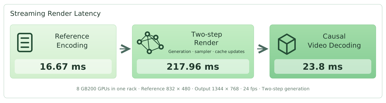
In the streaming loop. The decoder replaces only the video decoder of the pipeline; the TAE encoder for reference frames and the two-step DiT are unchanged. Its interface takes one latent frame at a time: the first latent frame of a pair is buffered, and when the second arrives the pair is decoded at once. At 768×1344 on the eight-GPU loop, the 32 ms version (before the KDA step) decodes 2 latent frames in 36.8–37.3 ms, against 264–329 ms for the DiT in the same round, and no block-start video frame differs from the VAE by more than two gray levels.
3.3Inference Acceleration and End-to-End Deployment
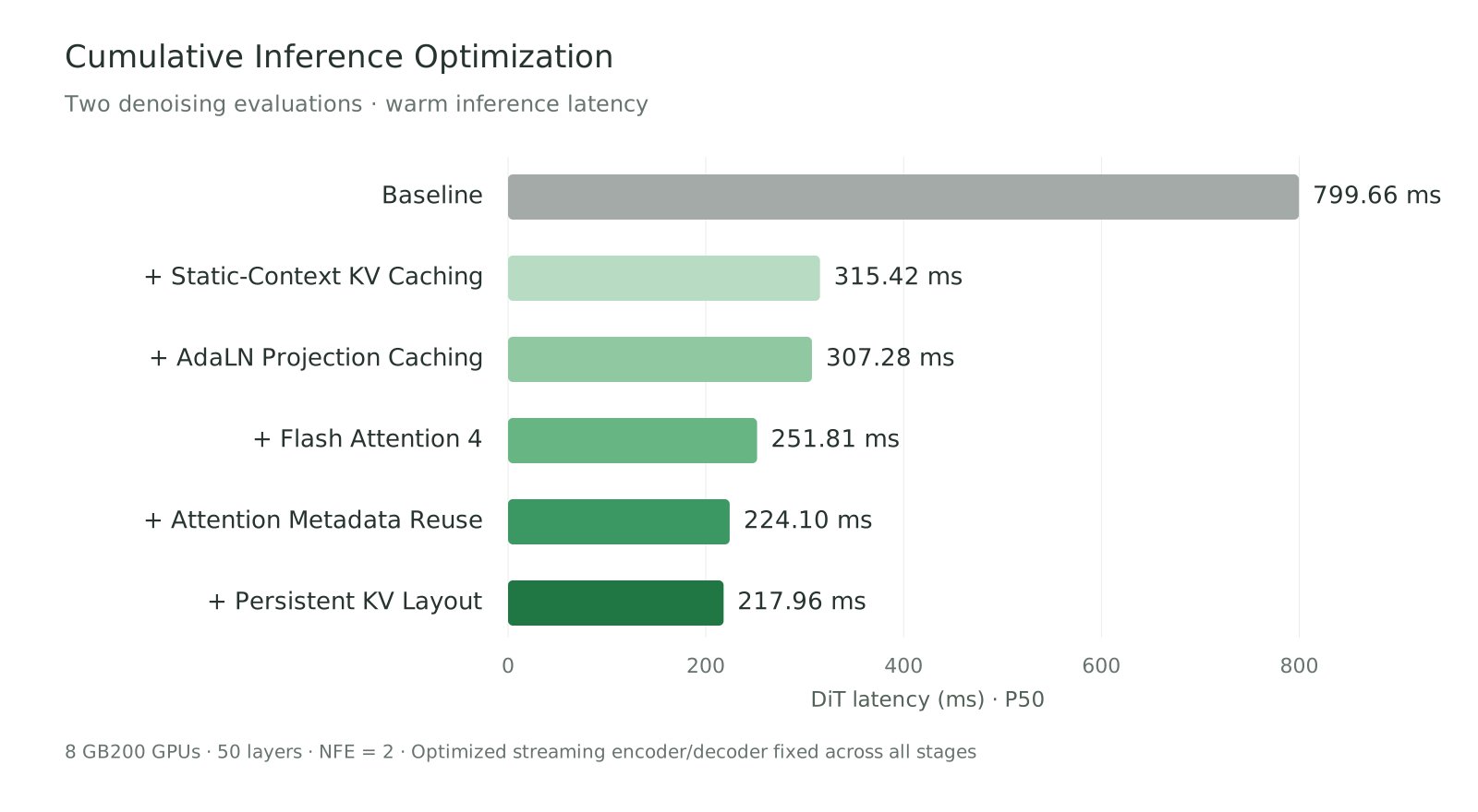
Real-time interaction requires every streaming step to return rendered frames within a tight latency budget. Starting from a PyTorch native baseline, we apply a series of complementary optimizations to the diffusion render, each removing a different source of redundant computation or data movement. The figure below shows their cumulative effect. The diffusion render time drops from 799.66 ms to 217.96 ms, a 3.67× speedup.
Multi-GPU parallel inference. To reach the lowest possible latency, we serve the model on eight GPUs. Each GPU keeps a full, resident copy of the model weights, so no weights are gathered or exchanged during inference. We split the work with Ulysses-style context parallelism. The token sequence of each streaming step is divided across the eight GPUs, and each GPU runs the feed-forward layers on its local shard. For attention, an all-to-all exchange regroups the data by head. Each GPU then attends over the full sequence for its subset of heads before the results return to the sequence layout.
Static-context KV caching. The context at each step falls into two parts. The static context holds the text–image conditioning features, the reference image, and the sink tokens. It stays fixed for the whole session. The dynamic context holds the current and most recent frames, and it changes as the stream moves forward. We compute the key/value states of the static context once and reuse them for every later chunk. Each denoising timestep keeps its own cache, so every step attends to context that matches it exactly. Each request reads directly from its own cache bank, which avoids any general-purpose merging along the way. Only the dynamic context is recomputed at each step. This greatly reduces the number of tokens processed by both the attention and feed-forward layers. This single change cuts the diffusion render time from 799.66 ms to 315.42 ms.
AdaLN projection caching. Each DiT block is conditioned through adaptive layer normalization (AdaLN). It projects the conditioning signal into the shift, scale, and gate parameters that modulate the block's activations. In streaming generation, the session conditioning is fixed and the denoising schedule repeats for every chunk. So the same inputs keep producing the same projections, layer after layer and chunk after chunk. We cache these projections and reuse them whenever the conditioning input is identical. Only the projection results are cached; the hidden activations, which change with every token, are left alone. This takes a repeated per-layer computation off the critical path and brings the diffusion render time further down to 307.28 ms.
Attention optimization. Splitting the model this finely across eight GPUs changes where the time goes. The feed-forward layers run locally on each shard and scale well. Attention, by contrast, combines the heaviest computation with cross-GPU communication and the most complex data movement. Under this parallel setup, attention becomes the largest remaining target for optimization, and we optimize it at three levels:
- Shape-aware kernel tuning. We run attention with a Blackwell-optimized FlashAttention-4 kernel and tune it for the exact query and key/value shapes that occur in streaming inference. Because each GPU handles a relatively small workload, we set the key/value split count to 1, avoiding the overhead of splitting. This reduces the diffusion render time from 307.28 ms to 251.81 ms.
- Attention metadata reuse. Besides queries, keys, and values, every attention call needs structural metadata: sequence lengths, cumulative offsets, and maximum lengths. Within one forward pass, layers that share the same sequence structure now prepare this metadata once and reuse it. This removes repeated per-layer setup and the host–device synchronization it caused, and lowers the diffusion render time to 224.10 ms.
- Persistent KV layout. Cached keys and values live in persistent per-layer buffers, stored directly in the layout the attention kernel reads. The static context is written once. Each step then updates only the dynamic region in place, which removes repeated memory allocation and history repacking. This brings the diffusion render time to its final 217.96 ms.
Together, these optimizations deliver real-time rendering across multiple GPUs, making interactive, real-time streaming video possible for users.
Current Limitations and Future Directions
One scenario so far. Everything reported here comes from the racing demo. The renderer, the two-step student, and the critics are trained only on racing data, with a third-person camera behind the player's car. The test drives come from the same game, so the models are fitted to this one scenario. The interface itself is not tied to racing, since any engine that can paint its scene with one flat color per class can drive the renderer. Covering more games and scenes, and measuring how much new data each one needs, is the next step.
A smaller, faster, sharper renderer. The streaming render still uses the full MiniMax-H3 DiT on eight GPUs. Reducing its parameter count, lowering the cost of each streaming step further, and improving the visual quality of the rendered video are the other directions we are pursuing.
Credits
Acknowledgements
We thank the teams and open projects that helped turn StreamRender-H3 from a code game engine and a video model into one real-time interactive world.
Core contributors
Yanzuo LuTian YeYitong LiShuchen XueHaozhe LiuSong HanEnze Xie
- MiniMaxMiniMax-H3 Ref2VA open weights and code, the base of the streaming renderer and the H3 VAE.
- LynnReal-OmniStreaming window with sink and recent history, and guidance fitting extended here to structure control.
- LongLiveFrame sink and streaming long tuning that our streaming DMD distillation follows.
- Humanize + KDAFused-kernel optimization of the Fast Causal H3 VAE decoder.
How to cite
Citations
If StreamRender-H3 helps your work, please cite this project page together with the underlying Sol-Engine paper.
@misc{streamrenderh3_2026,
  title        = {StreamRender-H3: Interactive Coding Worlds with Real-time Streaming Diffusion Render},
  author       = {Yanzuo Lu and Tian Ye and Yitong Li and Shuchen Xue and Haozhe Liu and Song Han and Enze Xie},
  year         = {2026},
  howpublished = {\url{https://nvlabs.github.io/Sana/Sol-Engine/StreamRender-H3/}},
  note         = {Project page}
}

@misc{li2026solvideoinferenceengine,
  title         = {Sol Video Inference Engine: Agent-Native Full-Stack Acceleration Framework for Efficient Video Generation},
  author        = {Yitong Li and Junsong Chen and Haopeng Li and Haozhe Liu and Jincheng Yu and Ligeng Zhu and Ping Luo and Song Han and Enze Xie},
  year          = {2026},
  eprint        = {2606.23743},
  archivePrefix = {arXiv},
  primaryClass  = {cs.CV},
  doi           = {10.48550/arXiv.2606.23743},
  url           = {https://arxiv.org/abs/2606.23743}
}