Installation#

Earth2grid has some compiled components (in CUDA and C). So some care is required to install. First, install pytorch, and setuptools

# python3 -m venv .venv # make venv
# source .venv/bin/activate # activate venv
pip install torch setuptools
pip install --no-build-isolation https://github.com/NVlabs/earth2grid/archive/main.tar.gz

Setup#

First, let’s import the necessary libraries and create a sample HealPIX grid.

#| label: setup
import matplotlib.pyplot as plt
import numpy as np
import torch

import earth2grid
from earth2grid import healpix

# Create a sample HealPIX grid
level = 3  # Resolution level (higher = finer resolution)
grid = healpix.Grid(level=level, pixel_order=healpix.PixelOrder.RING)
print(grid.lat[:5])

[84.14973294 84.14973294 84.14973294 84.14973294 78.28414761]

/Users/nbrenowitz/workspace/nvidia/earth2grid/earth2grid/healpix/core.py:112: UserWarning: healpixpad_cuda module not available, reverting to CPU for all padding routines
  warnings.warn("healpixpad_cuda module not available, reverting to CPU for all padding routines")

SHOW_AXES = False

def label_pixels(z):
    z = torch.as_tensor(z)
    npix = z.shape[0]
    i_ring = torch.arange(npix)
    nside = healpix.npix2nside(npix)
    y, x =healpix.ring2double(nside, i_ring)
    if label_pixels:
        for i in range(npix):
            plt.text((x[i] + nside).item() / 2, nside-(y[i] + 1).item() / 2, z[i].item(), ha='center', va='center', fontsize=12, color='white', clip_on=True)

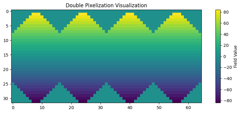
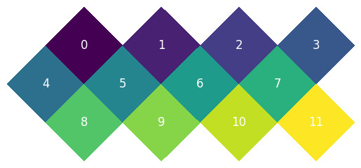
Visualization using Double Pixelization#

Double pixelization provides a visually appealing way to view HealPIX data without interpolation, preserving the native pixel structure. This is particularly useful for quick visualization with image viewers without distorting the native pixels of the image.

# Convert to double pixelization
field_double = healpix.to_double_pixelization(grid.lat)

plt.figure(figsize=(12, 4))
plt.imshow(field_double)
plt.colorbar(label='Field Value')
plt.title('Double Pixelization Visualization')
plt.show()

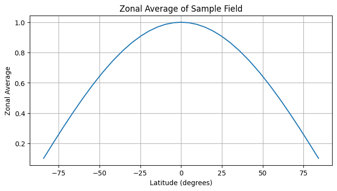
Zonal Averaging#

Zonal averaging computes the mean value of a field along latitude circles. This is useful for analyzing latitudinal patterns in the data.

# Compute the zonal average of the field
field = np.cos(np.deg2rad(grid.lat))
zonal_avg = healpix.zonal_average(field)
lat = healpix.zonal_average(grid.lat)

Show code cell source Hide code cell source

# Plot the zonal average
plt.figure(figsize=(8, 4))
plt.plot(lat, zonal_avg)
plt.xlabel('Latitude (degrees)')
plt.ylabel('Zonal Average')
plt.title('Zonal Average of Sample Field')
plt.grid(True)
plt.show()

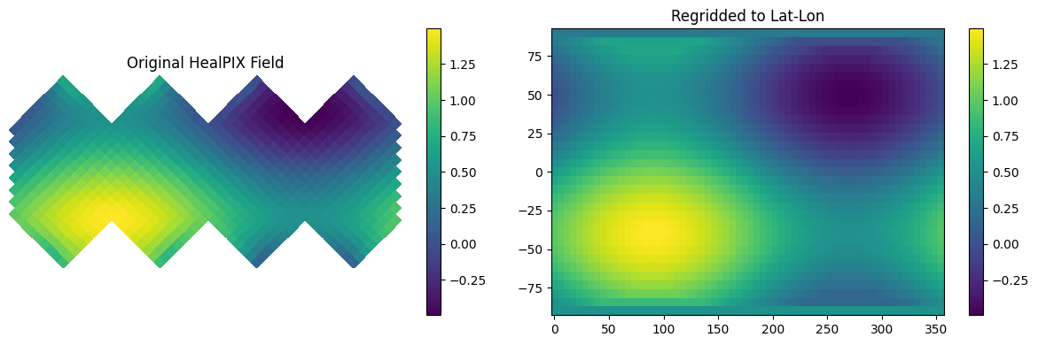
Regridding#

Regridding allows us to transform data between different grid types. Here we demonstrate two types of regridding:

1. From HEALPix to a regular lat-lon grid

2. Between HEALPix grids of different resolutions

Regridding to Lat-Lon#

earth2grid has builtin utilities for bilinear interpolation from any supported grid to arbitrary lat-lon points.

HEALPIX to Lat-Lon#

#| label: regrid-latlon
# Create a lat-lon grid
nlat, nlon = 33, 64
latlon_grid = earth2grid.latlon.equiangular_lat_lon_grid(nlat, nlon)

# Create regridder from HealPIX to lat-lon
regridder = earth2grid.get_regridder(grid, latlon_grid)

# Regrid the field
# must be a torch tensor
field = np.cos(np.deg2rad(grid.lat+ 40)) ** 2 + 0.5 * np.sin(np.deg2rad(grid.lon))
field_regridded = regridder(torch.from_numpy(field))

Show code cell source Hide code cell source

# Plot original and regridded fields
fig, (ax1, ax2) = plt.subplots(1, 2, figsize=(12, 4))

# Original HealPIX field
plt.sca(ax1)
im1 = healpix.pcolormesh(field)
ax1.set_title('Original HealPIX Field')
plt.colorbar(im1, ax=ax1)

# Regridded field
im2 = ax2.pcolormesh(latlon_grid.lon, latlon_grid.lat, field_regridded)
ax2.set_title('Regridded to Lat-Lon')
plt.colorbar(im2, ax=ax2)

plt.tight_layout()
plt.show()

A more verbose way, but flexible, way to do this is using the .get_bilinear_regridder_to method.

#| label: regrid-latlon-verbose

lat = np.linspace(-90, 90, 33)
lon = np.linspace(0, 360, 64)

regridder = grid.get_bilinear_regridder_to(lat[:, np.newaxis], lon[np.newaxis, :])
field_regridded = regridder(torch.from_numpy(field))
print(field_regridded.shape)

torch.Size([33, 64])

Note

Exercise: use get_bilinear_regridder_to to regrid to a list of unstructured points.

The regridding objects (and most operations in earth2grid) are fully differentiable and GPU capable

x = torch.randn(grid.shape)
x.requires_grad_(True)
regridder.to(x.dtype) # need to make sure the regridder is the same type as the input
y = regridder(x)
(y ** 2).sum().backward()
print(x.grad[:5])

tensor([ -4.0773,   0.4344, -20.1758, -24.9575, -12.2977])

from earth2grid import latlon
llgrid = latlon.LatLonGrid(lat=lat, lon=lon)
hpxgrid = healpix.Grid(level=6)
regridder = llgrid.get_bilinear_regridder_to(hpxgrid.lon, hpxgrid.lat)

field = lat[:, None] + 0 * lon # trick to get (nlat, nlon) array
out = regridder(torch.from_numpy(field))
print(out.shape)

torch.Size([49152])

HEALPix Pixel Orders#

earth2grid supports three main pixel ordering schemes:

• RING: Pixels are ordered in rings of constant latitude

• NEST: Pixels are ordered in a hierarchical, nested pattern

• XY: Pixels are ordered in a Cartesian-like grid within each face, with configurable origin and direction

The ability to reorder between these schemes is crucial for compatibility with different HEALPix implementations and for certain operations.

This is the default RING order:

Show code cell source Hide code cell source

def show_pixel_order(nside, pixel_order):
    npix = 12 * nside ** 2
    i = torch.arange(npix)
    ir = healpix.reorder(i, pixel_order, healpix.PixelOrder.RING)
    healpix.pcolormesh(ir)
    label_pixels(ir)
    if isinstance(pixel_order, healpix.XY):
        clockwise = pixel_order.clockwise
        plt.title(f"{pixel_order.origin.name}, {clockwise=}")

show_pixel_order(2, healpix.PixelOrder.RING)

And the NEST

Show code cell source Hide code cell source

show_pixel_order(2, healpix.PixelOrder.NEST)

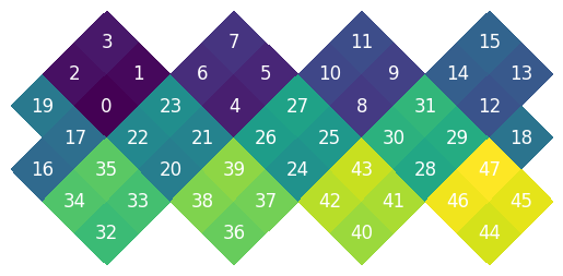
While NEST and RING are classic, we often want to treat each base pixel of the healpix grid as a 2d array. We have a XY pixel ordering object that allows us to do this.

Show code cell source Hide code cell source

def show_pixel_order(nside, pixel_order):
    npix = 12 * nside ** 2
    i = torch.arange(npix)
    ir = healpix.reorder(i, pixel_order, healpix.PixelOrder.RING)
    healpix.pcolormesh(ir.clamp(0, nside**2))
    label_pixels(ir)

    if isinstance(pixel_order, healpix.XY):
        clockwise = pixel_order.clockwise
        plt.title(f"XY(origin={pixel_order.origin.name}, {clockwise=})")
    else:
        plt.title(f"{pixel_order.name}")

nrow = 2
ncol = 2
plt.subplot(nrow, ncol, 1)
show_pixel_order(4, healpix.PixelOrder.NEST)
plt.ylim(0, 4)
plt.xlim(2, 6)

plt.subplot(nrow, ncol, 2)
show_pixel_order(4, healpix.XY())
plt.ylim(0, 4)
plt.xlim(2, 6)

plt.subplot(nrow, ncol, 3)
show_pixel_order(4, healpix.XY(origin=healpix.Compass.N, clockwise=False))
plt.ylim(0, 4)
plt.xlim(2, 6)

plt.subplot(nrow, ncol, 4)
show_pixel_order(4, healpix.XY(origin=healpix.Compass.N, clockwise=True))
plt.ylim(0, 4)
plt.xlim(2, 6)

(2.0, 6.0)

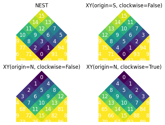
Why can convert between any two pixel orders like this:

healpix.reorder(x, healpix.PixelOrder.RING, healpix.PixelOrder.NEST) # ring to nest
healpix.reorder(x, healpix.PixelOrder.NEST, healpix.PixelOrder.XY()) # ring to XY

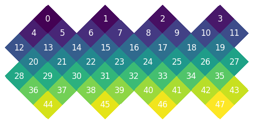
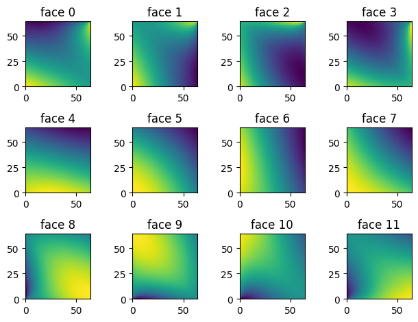
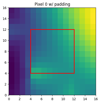
Padding and Convolutions#

The XY pixel order is useful for image analysis since it is a Cartesian-like grid. For example this is what the data looks like on each face of the sphere:

Show code cell source Hide code cell source

level = 6
nside = 2 ** level

grid = healpix.Grid(level)
field = np.cos(np.deg2rad(grid.lat+ 40)) ** 2 + 0.5 * np.sin(np.deg2rad(grid.lon))
field = torch.from_numpy(field)

out = healpix.reorder(field, healpix.PixelOrder.RING, healpix.XY())
faces = out.reshape([12, nside, nside])
for i in range(12):
    plt.subplot(3, 4, i+1)
    plt.pcolormesh(faces[i])
    plt.gca().set_aspect('equal')
    plt.title(f"face {i}")
plt.tight_layout()

Padding is a basic primitive for many machine learning methods. For example, convolutions un the sphere can be implemented as a padding followed by a convolution. Because of this we have written a CUDA padding routine that works for the HEALPix grid. It requires (origin=N, orientation=clockwise) i.e. [N, E, S, W]. For convenience we have an alias for this healpix.HEALPIX_PAD_XY. Let’s now call the padding routine and plot the padded region.

nside = 8
pad_size = 4

# Let's assume some data on the NEST grid (like is common for datasets)
grid = healpix.Grid(level=healpix.nside2level(nside), pixel_order=healpix.PixelOrder.NEST)
field = np.cos(np.deg2rad(grid.lat+ 40)) ** 2 + 0.5 * np.sin(np.deg2rad(grid.lon))
field = torch.from_numpy(field)

# now reorder, reshape and pad
out = healpix.reorder(field, grid.pixel_order, healpix.HEALPIX_PAD_XY)
z = out.reshape([1, 12, nside, nside]) # healpix.pad requires a 4d input
z_padded = healpix.pad(z, pad_size)

Show code cell source Hide code cell source

# show the padded region
import matplotlib.patches as patches
plt.pcolormesh(z_padded[0, 0])
rect = patches.Rectangle((pad_size, pad_size), nside, nside, linewidth=2, edgecolor='r', facecolor='none')
plt.gca().add_patch(rect)
plt.gca().set_aspect('equal')
plt.title("Pixel 0 w/ padding");

To run convolutions on the sphere

# convolution 3d is used to skip over the face dimension
conv = torch.nn.Conv3d(
  in_channels=1, out_channels=1, kernel_size=[1, 3, 3], padding=0
)

pad_size = 1
b, c, f, n, n = 1, 1, 12, nside, nside


x = out.view(b, c, f, n, n).float() # some input data

# start processing
y = x
y = y.view(b * c, f, n, n) # combine (b, c) dims, healpix.pad requires a 4d input
y = healpix.pad(y, pad_size)
y = y.view(b, c, f, n+2 * pad_size, n+2 * pad_size)
y = conv(y)
print(x.shape, y.shape)

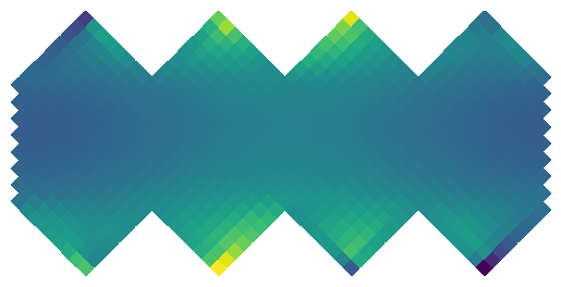
# reshape back for visualization
y = healpix.reorder(y.view(b, c, f * n  * n), healpix.HEALPIX_PAD_XY, healpix.PixelOrder.RING)
healpix.pcolormesh(y[0,0].detach())

torch.Size([1, 1, 12, 8, 8]) torch.Size([1, 1, 12, 8, 8])

<matplotlib.collections.QuadMesh at 0x12e5eb4d0>

Summary#

In this tutorial, we’ve covered several key aspects of working with HEALPix data:

1. Visualization: Using double pixelization to create visually appealing representations of HEALPix data while preserving the native pixel structure.

2. Zonal Averaging: Computing latitudinal averages to analyze patterns in the data.

3. Regridding: Transforming data between different grid types, including:

   • HEALPix to regular lat-lon grid

   • HEALPix to higher resolution HEALPix grid

4. Reordering: Converting between different HEALPix pixel ordering schemes:

   • RING: Pixels ordered in rings of constant latitude

   • NEST: Pixels ordered in a hierarchical, nested pattern

   • XY: Pixels ordered in a Cartesian-like grid within each face, with configurable origin and direction

5. Padding: Implementing efficient CUDA-based padding operations for machine learning applications, particularly useful for spherical convolutions.

These tools provide a comprehensive set of operations for working with global data on the sphere, making it easier to analyze, visualize, and process geophysical data for various applications including machine learning.