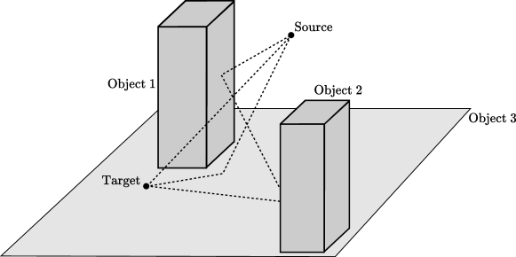
2 Essential Concepts and Terminology
2.1 Scene Objects and Meshes
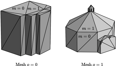
A scene object is represented as a mesh, which is composed of a set of triangles, also known as primitives, connected by their edges and vertices, as shown in Figure 3. Each object is identified by an index , and each primitive within an object is identified by an index . Each primitive possesses three edges, identified locally by an index . Primitives from different objects may share indices, therefore a primitive is uniquely identified by the pair . Similarly, an edge is uniquely identified by the triplet .
2.2 Rays and Paths
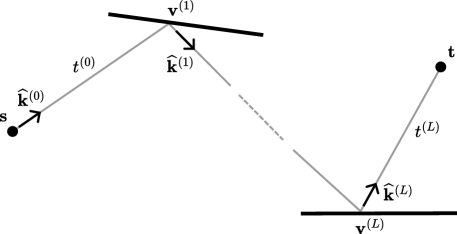
A ray is characterized by an origin , a direction , and a length . The direction is a unit vector, meaning . If the length is unspecified, the ray is considered infinite, i.e. . A path with depth is a sequence of rays that connect a source point to a target point , as illustrated in Figure 4,
| (6) |
where the superscript indicates the depth of the path, , , and . The ray origins together with the target are the path vertices. A path can therefore also be defined by a sequence of vertices:
| (7) |
In this case, the rays have directions and lengths for .
The suffix of a path, denoted by where , is defined as the sub-path consisting of all the rays from the -th one onward, i.e.
| (8) |
Similarly, the corresponding prefix is:
| (9) |
where corresponds to the empty path.
2.3 Interactions with Scene Objects
Sionna RT currently supports four types of interactions with scene objects:
- Specular reflection ():
-
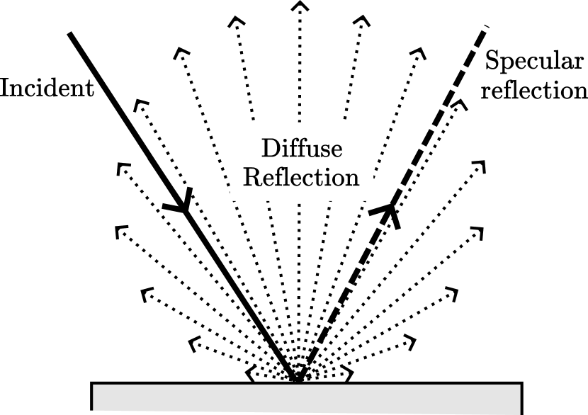
The wave is reflected with an angle of reflection equal to the angle of incidence, as illustrated in Figure 5(a).
- Diffuse reflection ():
-
The wave is reflected in multiple directions, as illustrated in Figure 5(a).
- Refraction ():
-
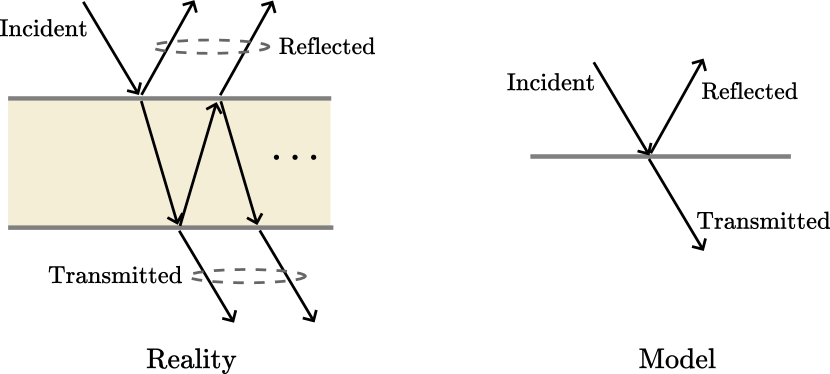
The wave propagates into the scattering medium. The solvers assume that object surfaces are thin enough that their effect on transmitted rays (i.e. rays that traverse the surfaces through double refraction) can be modeled by a single transmitted ray. The transmitted rays are traced without angular deflection. Surfaces like walls should be modeled as single flat surfaces, as illustrated in Figure 5(c). However, when computing the transmitted and reflected fields, the thickness of the traversed object is considered.
- Diffraction ():
-
The wave encounters a wedge-shaped object and is diffracted, as shown in Figure 5(b). Diffraction occurs in all directions along the Keller cone [10], where the angle between the incident ray and the wedge edge, denoted by , equals the angle between the diffracted ray and the wedge edge, denoted by . The wedge exterior angle is denoted by , such that . If the wedge’s exterior angle equals , i.e., , the wedge is termed an edge.
The set of possible interaction types is denoted by .

2.4 Ray Tubes
While a more detailed background on the propagation of EM waves is provided in Appendix A, we introduce here some essential EM concepts that are required for understanding the process of ray tracing. The source is modeled as a point source, an infinitesimally small emitter of EM waves that radiates in all directions according to a user-defined transmitter antenna pattern. Note that modeling transmit antennas as point sources is a valid approximation when the distances to scatterers and targets are significantly greater than the wavelength of the propagating waves. Each ray traced from the source serves as the axial ray of a ray tube [12, Chapter 2], which is a bundle of rays adjacent to the axial one. These ray tubes originate at the source and are characterized by a length and a solid angle (in steradians), as illustrated in Figure 6. Importantly, specular reflection and refraction through planar surfaces only alter the ray direction. Diffuse reflection and diffraction alter the shape of the wavefront. As detailed in Sections 3 and 4, this process requires specific computations to determine the path vertices and corresponding fields. For a given path with depth , we denote by the sequence of interaction types along the path. A key quantity for the remainder of this document is the depth of the last diffuse reflection, denoted by and defined as:
| (10) |
The dependency of on is omitted for brevity. The case where corresponds to paths that do not contain any diffuse reflection, known as specular chains. If , then the suffix is referred to as the specular suffix of . The value represents the depth index from which the path is composed solely of specular reflections, refractions, and diffraction, and is termed the specular suffix index of .