Wireless

This module provides blocks and functions that implement wireless channel models. Models currently available include AWGN, flat-fading with (optional) SpatialCorrelation, RayleighBlockFading, as well as models from the 3rd Generation Partnership Project (3GPP) [TR38901]: TDL, CDL, UMi, UMa, and RMa. It is also possible to use externally generated CIRs.

Apart from flat-fading, all of these models generate channel impulse responses (CIRs) that can then be used to implement a channel transfer function in the time domain or assuming an OFDM waveform.

This is achieved using the different functions, classes, and blocks which operate as shown in the figures below.

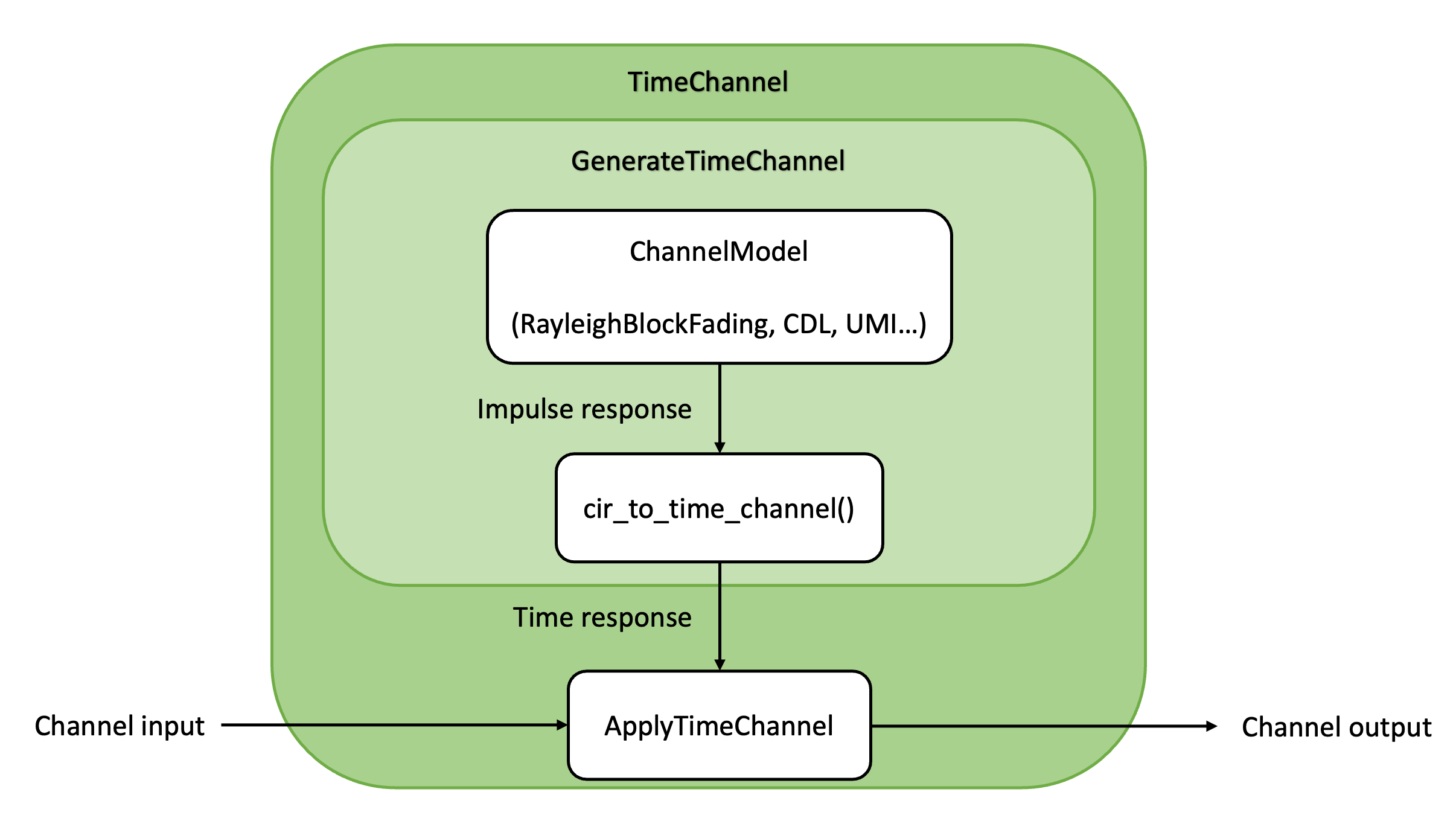
Fig. 10 Channel module architecture for time domain simulations.

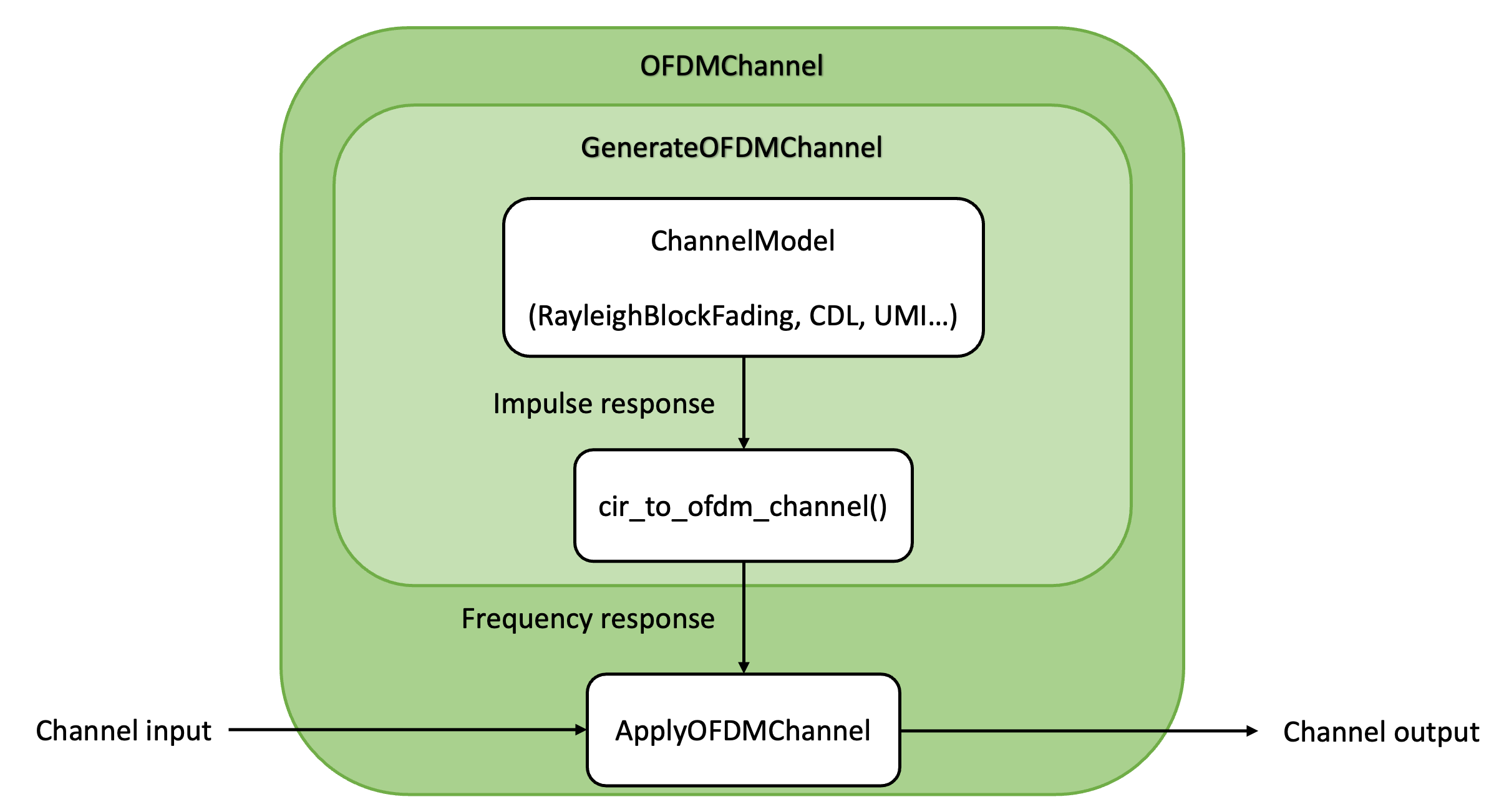
Fig. 11 Channel module architecture for simulations assuming OFDM waveform.

A channel model generate CIRs from which channel responses in the time domain or in the frequency domain are computed using the cir_to_time_channel() or cir_to_ofdm_channel() functions, respectively. If one does not need access to the raw CIRs, the GenerateTimeChannel and GenerateOFDMChannel classes can be used to conveniently sample CIRs and generate channel responses in the desired domain.

Once the channel responses in the time or frequency domain are computed, they can be applied to the channel input using the ApplyTimeChannel or ApplyOFDMChannel blocks.

The following code snippets show how to setup and run a Rayleigh block fading model assuming an OFDM waveform, and without accessing the CIRs or channel responses. This is the easiest way to setup a channel model. Setting-up other models is done in a similar way, except for AWGN (see the AWGN class documentation).

rayleigh = RayleighBlockFading(num_rx = 1,
                               num_rx_ant = 32,
                               num_tx = 4,
                               num_tx_ant = 2)

channel  = OFDMChannel(channel_model = rayleigh,
                       resource_grid = rg)

where rg is an instance of ResourceGrid.

Running the channel model is done as follows:

# x is the channel input
# no is the noise variance
y = channel(x, no)

To use the time domain representation of the channel, one can use TimeChannel instead of OFDMChannel.

If access to the channel responses is needed, one can separate their generation from their application to the channel input by setting up the channel model as follows:

rayleigh = RayleighBlockFading(num_rx = 1,
                               num_rx_ant = 32,
                               num_tx = 4,
                               num_tx_ant = 2)

generate_channel = GenerateOFDMChannel(channel_model = rayleigh,
                                       resource_grid = rg)

apply_channel = ApplyOFDMChannel()

where rg is an instance of ResourceGrid. Running the channel model is done as follows:

# Generate a batch of channel responses
h = generate_channel(batch_size)
# Apply the channel
# x is the channel input
# no is the noise variance
y = apply_channel(x, h, no)

Generating and applying the channel in the time domain can be achieved by using GenerateTimeChannel and ApplyTimeChannel instead of GenerateOFDMChannel and ApplyOFDMChannel, respectively.

To access the CIRs, setting up the channel can be done as follows:

rayleigh = RayleighBlockFading(num_rx = 1,
                               num_rx_ant = 32,
                               num_tx = 4,
                               num_tx_ant = 2)

apply_channel = ApplyOFDMChannel()

and running the channel model as follows:

cir = rayleigh(batch_size, num_time_steps, sampling_frequency)
h = cir_to_ofdm_channel(frequencies, *cir)
y = apply_channel(x, h, no)

where frequencies are the subcarrier frequencies in the baseband, which can be computed using the subcarrier_frequencies() utility function.

Applying the channel in the time domain can be done by using cir_to_time_channel() and ApplyTimeChannel instead of cir_to_ofdm_channel() and ApplyOFDMChannel, respectively.

For the purpose of the present document, the following symbols apply:

\(N_T (u)\)	Number of transmitters (transmitter index)
\(N_R (v)\)	Number of receivers (receiver index)
\(N_{TA} (k)\)	Number of antennas per transmitter (transmit antenna index)
\(N_{RA} (l)\)	Number of antennas per receiver (receive antenna index)
\(N_S (s)\)	Number of OFDM symbols (OFDM symbol index)
\(N_F (n)\)	Number of subcarriers (subcarrier index)
\(N_B (b)\)	Number of time samples forming the channel input (baseband symbol index)
\(L_{\text{min}}\)	Smallest time-lag for the discrete complex baseband channel
\(L_{\text{max}}\)	Largest time-lag for the discrete complex baseband channel
\(M (m)\)	Number of paths (clusters) forming a power delay profile (path index)
\(\tau_m(t)\)	\(m^{th}\) path (cluster) delay at time step \(t\)
\(a_m(t)\)	\(m^{th}\) path (cluster) complex coefficient at time step \(t\)
\(\Delta_f\)	Subcarrier spacing
\(W\)	Bandwidth
\(N_0\)	Noise variance

All transmitters are equipped with \(N_{TA}\) antennas and all receivers with \(N_{RA}\) antennas.

A channel model, such as RayleighBlockFading or UMi, is used to generate for each link between antenna \(k\) of transmitter \(u\) and antenna \(l\) of receiver \(v\) a power delay profile \((a_{u, k, v, l, m}(t), \tau_{u, v, m}), 0 \leq m \leq M-1\). The delays are assumed not to depend on time \(t\), and transmit and receive antennas \(k\) and \(l\). Such a power delay profile corresponds to the channel impulse response

\[h_{u, k, v, l}(t,\tau) = \sum_{m=0}^{M-1} a_{u, k, v, l,m}(t) \delta(\tau - \tau_{u, v, m})\]

where \(\delta(\cdot)\) is the Dirac delta measure. For example, in the case of Rayleigh block fading, the power delay profiles are time-invariant and such that for every link \((u, k, v, l)\)

\[\begin{split}\begin{aligned} M &= 1\\ \tau_{u, v, 0} &= 0\\ a_{u, k, v, l, 0} &\sim \mathcal{CN}(0,1). \end{aligned}\end{split}\]

3GPP channel models use the procedure depicted in [TR38901] to generate power delay profiles. With these models, the power delay profiles are time-variant in the event of mobility.