time_to_ofdm_channel#
- sionna.phy.channel.time_to_ofdm_channel(h_t: torch.Tensor, rg, l_min: int) torch.Tensor[source]#
Compute the channel frequency response from the discrete complex-baseband channel impulse response
Given a discrete complex-baseband channel impulse response \(\bar{h}_{b,\ell}\), for \(\ell\) ranging from \(L_\text{min}\) to \(L_\text{max}\), the discrete channel frequency response is computed as
\[\hat{h}_{b,n} = \sum_{\ell=L_\text{min}}^{L_\text{max}} \bar{h}_{b,\ell}e^{-j\frac{2\pi n\ell}{N}}, \quad n=0,\dots,N-1\]where \(N\) is the FFT size, \(b\) is the time step, \(n\) is the frequency-bin index, and \(\ell\) is the time-lag index. The FFT input stores the tap for lag \(\ell\) at index \(\ell \bmod N\).
This function only produces one channel frequency response per OFDM symbol, i.e., only values of \(b\) corresponding to the start of an OFDM symbol (after cyclic prefix removal) are considered.
- Parameters:
h_t (torch.Tensor) – Tensor of discrete complex-baseband channel impulse responses, shape […, num_time_steps, l_max-l_min+1]
rg – Resource grid
l_min (int) – Smallest time-lag for the discrete complex baseband channel impulse response (\(L_{\text{min}}\))
- Outputs:
h_f – […, num_ofdm_symbols, fft_size], torch.complex. Tensor of discrete complex-baseband channel frequency responses.
Notes
Note that the result of this function is generally different from the output of
cir_to_ofdm_channel()because the discrete complex-baseband channel impulse response is truncated (seecir_to_time_channel()). This effect can be observed in the example below.Examples
import matplotlib.pyplot as plt
import torch
from sionna.phy import config
from sionna.phy.channel import (subcarrier_frequencies,
    cir_to_ofdm_channel, cir_to_time_channel,
    time_lag_discrete_time_channel, time_to_ofdm_channel)
from sionna.phy.channel.tr38901 import TDL
from sionna.phy.ofdm import ResourceGrid

# Setup resource grid and channel model
config.seed = 42
rg = ResourceGrid(num_ofdm_symbols=1,
                  fft_size=1024,
                  subcarrier_spacing=15e3)
tdl = TDL("A", 100e-9, 3.5e9)

# Generate CIR
cir = tdl(batch_size=1, num_time_steps=1, sampling_frequency=rg.bandwidth)

# Generate OFDM channel from CIR
frequencies = subcarrier_frequencies(rg.fft_size, rg.subcarrier_spacing)
h_freq = cir_to_ofdm_channel(frequencies, *cir, normalize=True).squeeze()

# Generate time channel from CIR
l_min, l_max = time_lag_discrete_time_channel(rg.bandwidth)
h_time = cir_to_time_channel(rg.bandwidth, *cir, l_min=l_min, l_max=l_max, normalize=True)

# Generate OFDM channel from time channel
h_freq_hat = time_to_ofdm_channel(h_time, rg, l_min).squeeze()

# Compare the two frequency responses
plt.figure(figsize=(7, 5))
plt.plot(h_freq.real.cpu(), label="OFDM channel (real)")
plt.plot(h_freq_hat.real.cpu(), "--",
         label="OFDM channel from time (real)")
plt.plot(h_freq.imag.cpu(), label="OFDM channel (imag)")
plt.plot(h_freq_hat.imag.cpu(), "--",
         label="OFDM channel from time (imag)")
plt.xlabel("Subcarrier index")
plt.ylabel("Channel frequency response")
plt.grid()
plt.legend()
plt.show()
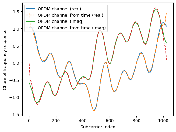
Fig. 24 Frequency responses computed directly from the CIR and from the truncated discrete time channel.#