Bilateral and Permutohedral Filters
Created: 2026-04-30 19:55:27 PST Edited: 2026-05-03 12:00:00 PST
WarpConvNet ships three families of edge-preserving filters for point clouds and high-dimensional feature volumes. They differ in the underlying spatial data structure and trade off accuracy vs. cost differently. All three share the same separation between lattice coordinates (the bilateral guide: typically xyz + color) and the feature being filtered (color, labels, depth, anything per-point).
Why bilateral filters live in WarpConvNet
A bilateral filter is a spatially sparse convolution in a high-dimensional space. The 3D voxel sparse convolution from Spatially Sparse Convolutions operates on \(\mathcal{C} \subset \mathbb{Z}^3\); a bilateral filter operates on \(\mathcal{C} \subset \mathbb{Z}^{d_{\text{xyz}} + d_{\text{feat}}}\) where the extra axes encode range features (color, intensity, time). The bilateral guide is the lift into that high-D integer grid:
Two pixels with similar color end up at neighboring high-D coordinates and are summed; two pixels with the same xy but different color sit far apart in the lift and don't interact — this is what makes the filter edge-preserving.

Left: a 1D signal with two intensity regions and a sharp edge at \(x{=}0.5\). Right: the 2D bilateral lift \((x/\sigma_x,\,I/\sigma_I)\). Points across the edge are spatially adjacent in \(x\) but separated by a wide gap in \(I/\sigma_I\), so the lifted convolution kernel never bridges them.
The same spatial sparsity that makes 3D voxel convolutions tractable is what makes high-D bilateral filtering tractable: even though the lifted grid has \(\sim 10^{10}\) cells at \(d{=}6\), only the cells touched by input points are materialized. The same building blocks back both:
| Voxel sparse conv (3D) | Bilateral / permutohedral filter (high-D) |
|---|---|
| Coords: \((b, x, y, z) \in \mathbb{Z}^4\) | Coords: \((b, x, y, z, r, g, b) / \sigma \in \mathbb{Z}^{\le 8}\) |
Hash: PackedHashTable (64-bit, 18 bits per axis) |
Hash: PackedHashTable128 (128-bit, 17 bits per axis, \(D \le 7\)) |
| Kernel-map build → gather–GEMM–scatter | Splat (gather) → separable blur → slice (scatter) |
| Kernel offsets \(\mathcal{K} \subset \mathbb{Z}^3\) (\(3^3\), \(5^3\), \(\ldots\)) | Separable 3-tap Gaussian along each of \(d\) (grid) or \(d{+}1\) (permutohedral) axes |
Splat–blur–slice is sparse convolution. Splat is the gather phase from
spatially_sparse_conv; the blur is a
depthwise sparse convolution applied separably along each lattice axis
(the kernel weights are fixed Gaussian taps \([\tfrac14, \tfrac12, \tfrac14]\)
rather than learned, but the data motion is identical to
spatially_sparse_depthwise_conv); slice is the
scatter back to per-point queries. The permutohedral variant additionally
projects to a \((d{+}1)\)-D simplicial lattice so neighbor count per cell is
\(d{+}1\) instead of \(2^d\) — same idea, different tessellation.

The three-stage pipeline on a 2D lifted grid. (a) Splat: a query distributes its value to the \(2^d{=}4\) corners of its enclosing cell with bilinear weights \(w_{ij}\). (b) Blur: a separable 3-tap Gaussian sweeps each lattice axis over only the populated cells — this is exactly a depthwise sparse convolution with fixed kernel taps. (c) Slice: the filtered cell values are bilinearly gathered back to the query point with the same weights as splat.
The permutohedral lattice swaps the cube tessellation for a simplicial one, shrinking neighbor count per cell from \(2^d\) to \(d{+}1\):

Left: a \(d{=}2\) query splatting to a cube cell needs \(2^d{=}4\) corner
updates; the same query in a simplicial cell needs \(d{+}1{=}3\) vertex
updates. Right: the populated permutohedral lattice is stored sparsely in
PackedHashTable128 — empty triangles are never
materialized. The savings compound rapidly with \(d\): at \(d{=}6\), \(2^d{=}64\)
vs. \(d{+}1{=}7\).
This is why bilateral filters ship with WarpConvNet rather than as a
separate package: they reuse the
PackedHashTable128 coordinate index, the same
gather/scatter primitives as voxel convolutions, and the same CUDA build
infrastructure. If you already have a sparse-convolution pipeline, the
bilateral filter is the same machinery applied to a higher-dimensional
lattice.
When to use which
| Filter | Backend | \(d\) supported | Best for |
|---|---|---|---|
BilateralFilter |
KNN / radius | any | \(\le 100\)k points, exact Gaussian, predictable memory |
BilateralFilterGrid |
sparse \(d\)-cube | \(D_{\text{xyz}} + D_{\text{feat}} \le 6\) | \(d\) small (\(\le 4\)), regular sampling |
BilateralPermutohedralFilter |
permutohedral lattice | \(D_{\text{xyz}} + D_{\text{feat}} \le 6\) | high \(d\) (5–6), irregular point clouds |
For typical bilateral on RGB point clouds (\(d_{\text{xyz}} = 3\), \(d_{\text{feat}} = 3\), total 6), the permutohedral lattice is canonical and fastest. For low-\(d\) guidance (\(d \le 4\), e.g. depth + xy) the regular \(d\)-cube grid is simpler and a touch faster on dense data.
The fast bilateral solver lives on top of BilateralGrid for confidence-weighted
smoothing.
Lattice coordinates vs. value
Every filter takes two roles for input tensors:
- Lattice coordinates (the bilateral guide): combined position + range features, scaled by per-axis bandwidths \(\sigma\). xyz alone collapses the filter to a plain spatial Gaussian; appending color gives edge-preserving bilateral semantics.
- Value (
src_value): the per-point quantity being splatted, blurred, and sliced. Independent of the guide. Pass the same tensor assrc_featandsrc_valueto denoise color; pass labels (one-hot) assrc_valueto propagate labels along the bilateral kernel.
The guide is what determines which points get averaged together. The value is what gets averaged. They can be the same tensor, different tensors, or partially overlap.
BilateralFilter — KNN / radius
Direct \(K\)-neighbor Gaussian aggregation per query, no lattice. Memory proportional to \(K \cdot N\). Use when \(N\) is moderate and you want bit-exact Gaussian weights without lattice approximation error.
import warpconvnet.nn as wn

filt = wn.BilateralFilter(
    sigma_xyz=0.05, sigma_feat=20.0,
    k=16, mode="knn",          # or mode="radius"
)
out = filt(src_xyz, src_feat, src_value)
For each query point, pulls the \(K\) spatial neighbors via WarpConvNet's
chunked KNN, weights each by \(\exp(-\lVert\Delta\mathrm{xyz}\rVert^2 /
2\sigma_{\text{xyz}}^2 - \lVert\Delta\mathrm{feat}\rVert^2 /
2\sigma_{\text{feat}}^2)\), and returns the weighted mean. mode="radius"
swaps fixed-\(K\) for a \(3\sigma_{\text{xyz}}\) ball; lower work per query
on highly non-uniform densities.
Companion: bilateral_label_propagate densifies sparse labels by
bilateral-weighted voting across each query's \(K\) neighbors, restricted
to non-background sources.
BilateralFilterGrid — sparse \(d\)-cube
Splats each input to the \(2^d\) corners of its enclosing voxel with
\(d\)-linear barycentric weights, blurs with separable 3-tap kernels along
each of the \(d\) axes, slices back. Sparse storage: only voxels touched by
at least one input are materialized — exactly the spatial-sparsity regime
of spatially_sparse_conv, lifted from \(D{=}3\)
to \(D = d_{\text{xyz}} + d_{\text{feat}}\). The blur is a fixed-weight
depthwise sparse convolution; if you replaced the Gaussian taps with
learned weights you would recover a high-D learned sparse convolution.
filt = wn.BilateralFilterGrid(sigma_xyz=0.05, sigma_feat=20.0)
out = filt(src_xyz, src_feat, src_value)
Lattice coordinates: concat([src_xyz / sigma_xyz, src_feat / sigma_feat]).
Total dimensionality must satisfy \(d_{\text{xyz}} + d_{\text{feat}} \le 6\)
(the PackedHashTable128 budget is \(D = 7\) axes).
Build once, filter many features:
filt = wn.BilateralFilterGridCached(sigma_xyz=0.05, sigma_feat=20.0)
filt.build_grid(src_xyz, src_feat)
out_rgb    = filt(rgb)
out_labels = filt(label_onehot)
BilateralPermutohedralFilter — permutohedral lattice
The Adams–Baek–Davis (2010) lattice. Each input embeds into a \((d+1)\)-D
simplicial lattice; its feature distributes across the \((d{+}1)\) vertices
of the enclosing simplex with barycentric weights. Blur is a separable
3-tap Gaussian along each of the \((d{+}1)\) lattice axes — i.e.
\(d{+}1\) depthwise sparse convolutions on the populated lattice vertices,
indexed by the same PackedHashTable128 used for
3D voxel kernel maps. The simplicial tessellation is what makes the
neighbor count \(d{+}1\) instead of the \(d\)-cube's \(2^d\), killing the
exponential blow-up that limits BilateralFilterGrid past \(d{=}4\).
Complexity: \(O(N \cdot d^2)\) for splat/slice and \(O(V \cdot d^2)\) for blur where \(V \le N(d{+}1)\) is the number of unique populated lattice vertices.
filt = wn.BilateralPermutohedralFilter(sigma_xyz=0.05, sigma_feat=20.0)
out = filt(src_xyz, src_feat, src_value)
# Cross-position (filter at different sites than build):
out = filt(src_xyz, src_feat, src_value, query_xyz, query_feat)
Cached variant for iterative use:
filt = wn.BilateralPermutohedralFilterCached(sigma_xyz=0.05, sigma_feat=20.0)
filt.build_lattice(src_xyz, src_feat)
out1 = filt(rgb)
out2 = filt(rgb_modified)
For full control over per-axis bandwidths or pre-scaled positions, the low-level functional API is also exposed:
from warpconvnet.nn.functional.permutohedral import permutohedral_filter
out = permutohedral_filter(positions, features, sigmas=[16, 16, 12, 12, 12, 1])
FastBilateralSolver — Barron–Poole 2015
Confidence-weighted smoothing built on top of BilateralGrid:
Solved in grid space via PCG with a Jacobi preconditioner; result is sliced back to per-input estimates. Useful for depth super-resolution, label propagation with a data term, or any noisy observation \(t\) with per-point confidence \(c\).
solver = wn.FastBilateralSolver(
    sigma_xyz=0.05, sigma_feat=20.0,
    lam=128.0, max_iters=25, tol=1e-5,
)
smoothed = solver(src_xyz, src_feat, target, confidence)
Sinkhorn-style bistochastization runs by default; disable via the
underlying bilateral_solver(grid, ..., bistochastize=False) if extreme
confidence values cause non-finite scaling factors.
Worked example: 2D image denoising
Image denoising is the canonical bilateral demo: each pixel is a point with
a 2D position and a 3D color, the guide is concat(xy/sigma_xy, rgb/sigma_rgb), and the value being filtered is the noisy color itself.
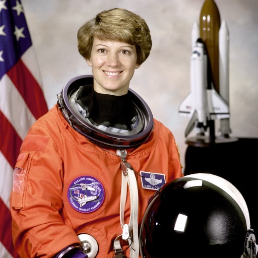
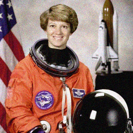
The example below applies all three filter families to the NASA astronaut
test image (public domain, shipped with scikit-image) corrupted with
Gaussian noise of variance 0.01. End-to-end times are on an RTX 6000 Ada at
512×512 = 262k "points" with \(\sigma_{xy} = 4\), \(\sigma_{rgb} = 0.1\).
Input
| Original | Noisy (Gaussian, var=0.01) — 20.70 dB |
 |
 |
Output
| KNN (k=24) — 23.67 dB / ~3.3 s | Grid — 23.94 dB / ~63 ms | Permutohedral — 24.68 dB / ~11 ms |
 |
 |
 |
| Filter | Time | PSNR (dB) | Notes |
|---|---|---|---|
| Noisy input (reference) | — | 20.70 | Gaussian noise, var = 0.01 |
BilateralFilter (KNN, k=24) |
~3.3 s | 23.67 | Exact Gaussian, \(O(N \cdot k)\) |
BilateralFilterGrid |
~63 ms | 23.94 | \(d=5\) sparse cube |
BilateralPermutohedralFilter |
~11 ms | 24.68 | \(d=5\) permutohedral lattice |
PSNR is computed against the clean original with data_range=1.0. The
permutohedral lattice is both fastest and highest PSNR here — its
conservative reconstruction (3-tap Gaussian on \((d{+}1)\) lattice axes)
preserves edges slightly better than the \(d\)-cube grid at this bandwidth,
and noticeably better than the limited-\(K\) KNN filter where boundary
neighbors get clipped.
Reproduce with examples/demos/bilateral_image.py:
python examples/demos/bilateral_image.py \
    --out-dir docs/user_guide/img \
    --sigma-xy 4.0 --sigma-rgb 0.1 --noise-var 0.01
Sketch of the call site:
from skimage import data, util
import torch
import warpconvnet.nn as wn

img = util.img_as_float(data.astronaut())                    # (512, 512, 3)
noisy = util.random_noise(img, mode="gaussian", var=0.01)
h, w, _ = img.shape

ys, xs = torch.meshgrid(torch.arange(h), torch.arange(w), indexing="ij")
xy  = torch.stack([xs, ys], dim=-1).reshape(-1, 2).float().cuda()
rgb = torch.from_numpy(noisy).reshape(-1, 3).float().cuda()

filt = wn.BilateralPermutohedralFilter(sigma_xyz=4.0, sigma_feat=0.1)
denoised = filt(xy, rgb, rgb).reshape(h, w, 3).clamp(0, 1)
The KNN filter is exact-Gaussian but \(O(N \cdot k)\); the lattice variants trade ~10–20% reconstruction error for two orders of magnitude in speed and become the only viable option above ~\(10^5\) points.
Constraints
PackedHashTable128supports \(D \le 7\) axes per key. Lattice dimensionality (xyz + feat for grid; \(d{+}1\) lattice axes for permutohedral) must fit. Practically, \(d_{\text{xyz}} + d_{\text{feat}} \le 6\).- Coords pack with 17 bits per axis \(\Rightarrow\) each component must lie
in \([-65536, 65535]\) after sigma scaling. Outside this range the lattice
coordinate silently truncates unless
WARPCONVNET_DEBUG_HASH=1is set. - All inputs must be CUDA tensors; CPU paths are not implemented.
Performance notes
Hero benchmark (RGB d=6, RTX 6000 Ada)
For \(N = 196{,}608\) pixels, \(d = 6\) (xyz pixel coords + RGB), \(F = 3\) features filtered, sigmas \(= [16, 16, 12, 12, 12, 1]\):
| Stage | Time (ms) |
|---|---|
| build (lattice + hash table) | 4.07 |
| splat | 0.12 |
| blur | 2.54 |
| slice | 0.05 |
total filter() |
7.20 |
filter() takes ~24% of its time in build; for iterative bilateral
(e.g., a 25-iteration solver over fixed positions) prefer the Cached
variants and amortize the build over all calls.
Pad-channel optimization
Internal: filter() pads the post-splat lattice from \(C\) to \(C{+}1\)
channels when \(C\) is divisible by 4, runs splat–blur–slice on the
padded width, strips the pad column at the end. This sidesteps a torch
gather kernel pessimum at \(C \in \{4, 8, 12, 16, 20, \ldots\}\)
(observed on torch 2.10.0+cu128, ~10–15× slower than \(C{=}3\) for
random-index gather). The padded column is zero throughout linear ops
so the math is identical.
The most common consumer hits the cliff exactly: RGB filter with homogeneous normalization splats \(F{+}1 = 4\) channels per vertex. Without the pad workaround, blur on this width is ~12 ms instead of ~2.5 ms.
The workaround is version-locked. On torch upgrade, re-run the C-sweep
in tests/nn/bench_permutohedral_d6.py (extend it) and the inline
notes in warpconvnet/nn/functional/permutohedral.py. If the cliff is
gone the pad path can be removed.
See also
- Spatially Sparse Convolutions — the 3D voxel analog. Bilateral filters are the same gather → kernel-apply → scatter pipeline lifted to a higher-dimensional lattice with fixed Gaussian weights instead of learned ones.
- Packed Hash Table — the coordinate index that
backs both voxel sparse conv (
PackedHashTable, 64-bit) and the lattice filters here (PackedHashTable128, 128-bit, \(D \le 7\)). - Point Convolutions — continuous-coordinate
alternative for the KNN/radius regime; what
BilateralFilter(modeknn/radius) reduces to with Gaussian weights.
Source
warpconvnet/nn/functional/bilateral.py(KNN / radius)warpconvnet/nn/functional/bilateral_grid.py(regular grid + solver)warpconvnet/nn/functional/permutohedral.py(lattice)warpconvnet/nn/modules/bilateral.pywarpconvnet/nn/modules/permutohedral.pywarpconvnet/geometry/coords/search/packed128_hashmap.py(PackedHashTable128, used by both lattice variants; handleskey_dim < 7via internal zero-pad)
References
- Adams, A., Baek, J., Davis, M. A. Fast High-Dimensional Filtering Using the Permutohedral Lattice (2010).
- Barron, J. T., Poole, B. The Fast Bilateral Solver (arXiv:1511.03296).
- Tomasi, C., Manduchi, R. Bilateral Filtering for Gray and Color Images (ICCV 1998) — original definition.