Voxel Size Caveats: Detail Loss vs. Point Continuity
Spatially sparse convolutions only see what falls into a voxel cell, and only exchange information with neighbors covered by the kernel footprint. Voxel size sits at the heart of both of those constraints, so the choice has two failure modes that pull in opposite directions:
| Voxel too large | Voxel too small |
|---|---|
| Distinct geometry collapses into the same cell. Detail destroyed before the network ever sees it. | Most cells contain ≤1 point, neighbors no longer fall inside each other's kernel footprint. Convolutions stop exchanging information. |
This page uses a 2-D two-moons toy dataset to make both failure modes visible. The same intuitions transfer directly to 3-D point clouds.
All figures are generated by
docs/user_guide/scripts/voxel_size_caveats_figures.py. Re-run that script to regenerate them.
1. The dataset
We use two interlocking half-circles ("moons"), 400 noisy points per class. Class A in red (●), Class B in blue (▲). They are linearly inseparable but geometrically obvious.
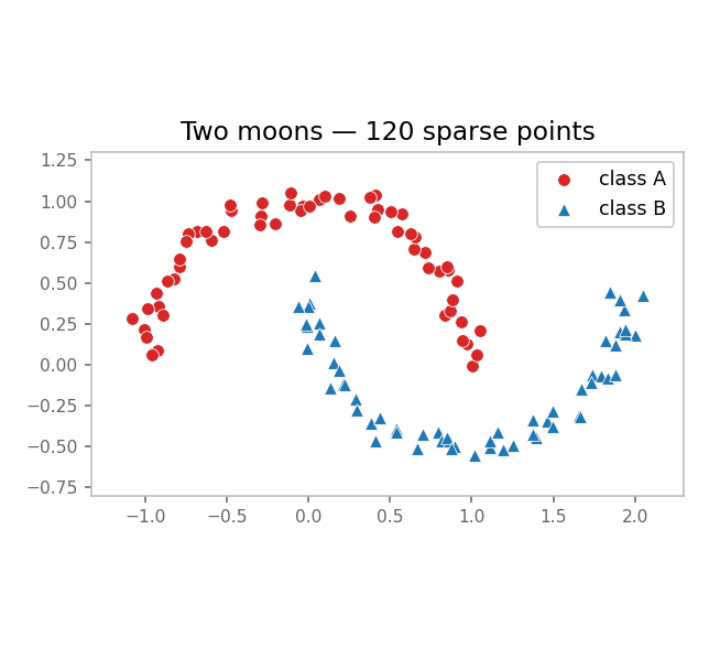
A trained 2-D sparse-conv classifier needs to see the curvature of each moon to separate them. Anything that destroys that curvature kills accuracy.
2. Failure mode 1 — voxel too large: detail collapses
Drop the same points into three different grids:
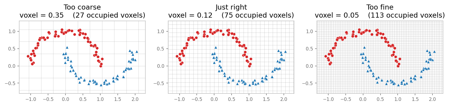
Now look at what the convolution actually sees — voxel cells colored by the majority class inside (or by red/blue mixing ratio for the coarse case):
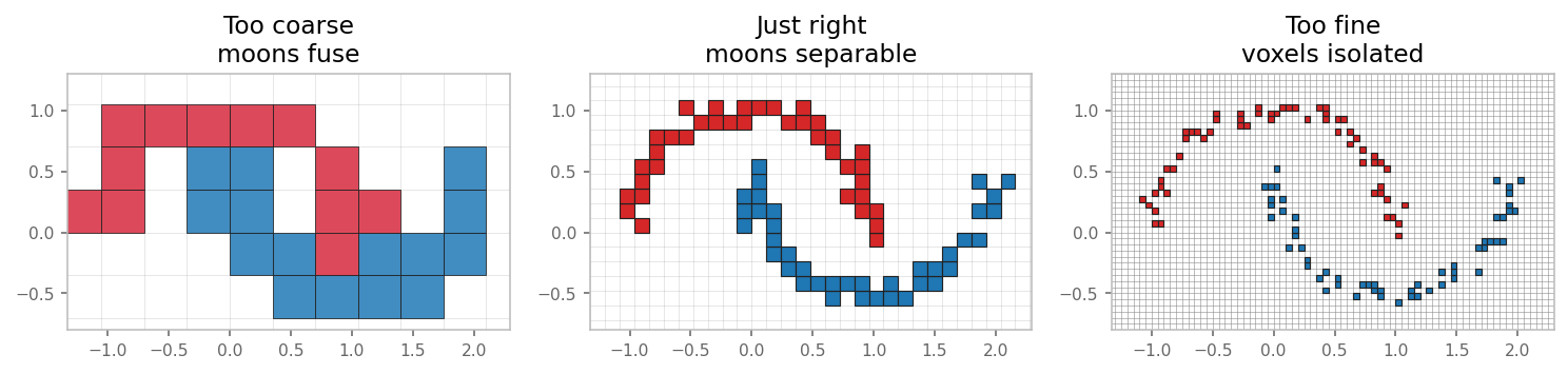
- Too coarse (voxel = 0.35). A single voxel covers a chunk of both moons. The cell ends up muddled (purple = mixed red/blue inside one cell). No downstream network can recover the moon shape from these inputs because the information was thrown away during voxelization.
- Just right (voxel = 0.12). Each cell sits inside one moon. The two curves stay clearly separable.
- Too fine (voxel = 0.05). Each occupied cell holds ~1 point. Looks fine in isolation — but see the next section for what breaks.
Rule of thumb. Voxel size should be smaller than the smallest feature you need to distinguish. For ScanNet at 0.02 m, the smallest feature is roughly the thickness of a chair leg.
3. Failure mode 2 — voxel too small: kernels stop overlapping
A 3×3 sparse convolution at voxel v reads features from every voxel within
Chebyshev distance ≤ 1 of v. Two voxels can exchange information only if
one falls inside the other's 3×3 kernel footprint.
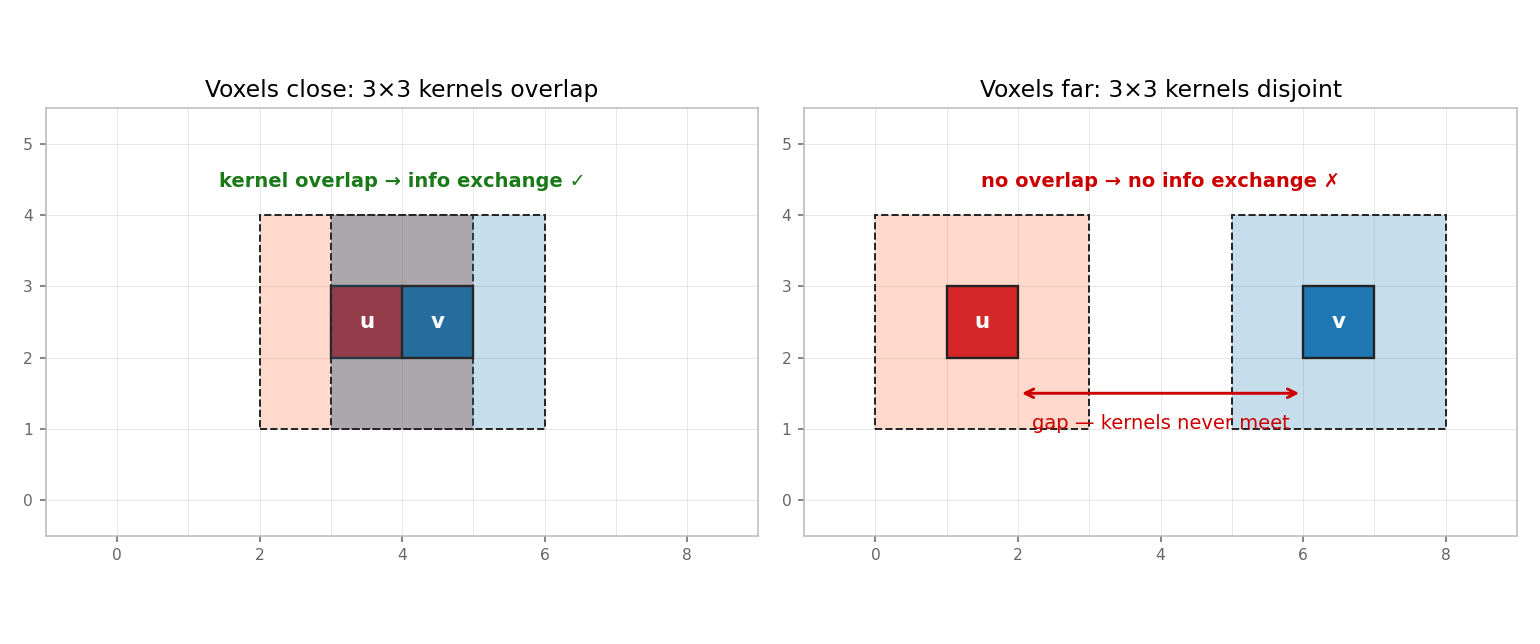
- Left. Voxels
uandvare adjacent. Their 3×3 footprints overlap (gray region). One conv layer is enough to mix their features. ✓ - Right. Voxels
uandvare 4 cells apart. Their 3×3 footprints are disjoint. A single conv layer cannot pass information between them, no matter what kernel weights you train. ✗
When the voxel size is much smaller than the typical inter-point spacing, most voxels look like the right panel. The sparse conv is mathematically defined but operationally trivial — the kernel only ever sees one voxel at a time, so it degenerates into a per-voxel MLP.
The connectivity graph at voxel size 0.12 vs. 0.05 makes this concrete. Each edge means "these two voxels are 1-hop neighbors under a 3×3 kernel":
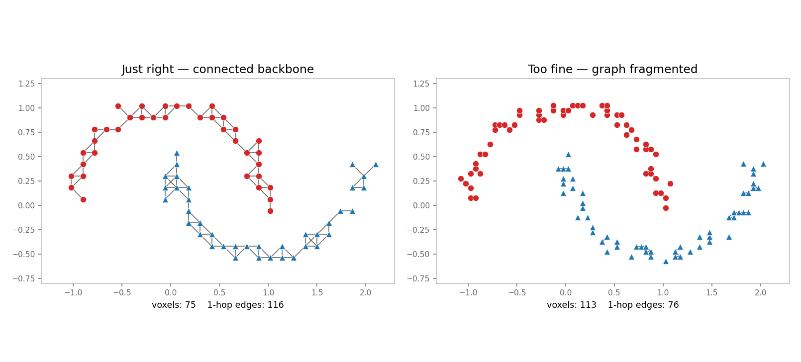
- Just right (left). A connected backbone runs along each moon. A few conv layers spread information along the entire curve.
- Too fine (right). Edge count collapses. The graph fragments into isolated voxels and tiny clumps. Information cannot flow.
This is the point-continuity issue: in dense 2-D images, every pixel has a neighbor in every direction. In sparse 3-D, neighborhood is emergent from the data density — make voxels too small and the neighborhood disappears.
4. The receptive-field tradeoff
The two failure modes are coupled through the receptive field. The
receptive field of L stacked 3×3 convolutions is (2L+1) voxels wide.
Halve the voxel size, and the world-space coverage of the same network
also halves:
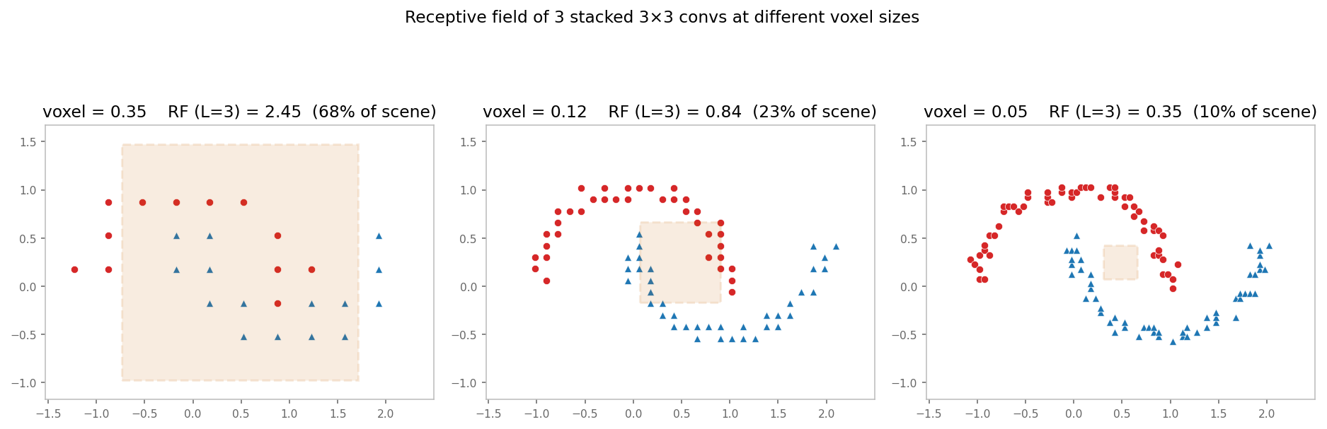
In the rightmost panel, the orange box is the receptive field of three 3×3 convs at voxel = 0.05. It barely covers a fraction of one moon, so even if the connectivity graph is healthy, the network needs many more layers (or strided downsampling) to see global structure.
At voxel = 0.35 the receptive field exceeds the scene — but you already discarded the detail you wanted to recognize.
5. Practical guidance
- Pick voxel size from the data, not from the model. Start from the smallest geometric feature you must preserve. A common heuristic for 3-D indoor scans is 0.02–0.05 m; for outdoor LiDAR, 0.05–0.20 m.
- Sanity-check connectivity. After voxelization, count edges in the 1-hop graph. If most voxels have \<3 neighbors, your voxel size is small compared to your point density — either upsample, increase the voxel size, or use kernel size > 3.
- Increase kernel size before shrinking voxel size. Going from a 3³ kernel to a 5³ kernel doubles the per-layer reach in voxel space without destroying detail. Going to a smaller voxel size shrinks reach.
- Use strided downsampling. Encoder–decoder networks (MinkUNet, etc.) start at the finest resolution and downsample to recover global context without sacrificing the early-layer detail.
- Concatenate raw point features. When per-voxel pooling is unavoidable
but you still want sub-voxel detail, propagate per-point features through
PointToVoxel(..., concat_unpooled_pc=True)so the decoder sees both voxel- and point-level information.
6. Reproducing the figures
source .venv/bin/activate
python docs/user_guide/scripts/voxel_size_caveats_figures.py
Outputs land in docs/user_guide/img/voxel_caveats/. The script depends
only on numpy and matplotlib (no sklearn), so it runs in any
warpconvnet venv.