Dense-CRF Mean-Field as Sparse Convolution¶
Created: 2026-05-03 19:42:26 PST Edited: 2026-05-03 19:42:26 PST
A dense Conditional Random Field (CRF) over image pixels — every pixel connected to every other pixel — is, at first sight, intractable: with \(N = HW\) pixels and \(K\) labels, message passing costs \(O(N^2 K)\). Krähenbühl & Koltun (2011) showed that when the pairwise potential is a Gaussian in some feature space, mean-field inference reduces to filtering with that Gaussian — and high-dimensional Gaussian filtering reduces to a sparse convolution on a lattice in that high-dimensional space.
This page reproduces their dense-CRF on a 2D image using the same primitives
WarpConvNet uses for 3D and higher. The 5D appearance kernel is the
interesting bit; the 2D smoothness kernel is honest dense Conv2d. The
example ships as
examples/demos/crf_image.py.
The paper's full trilateral construction (7D, RGB videos) is the same idea in higher dimension; see Going higher: 7D trilateral CRF.
Model¶
Each pixel \(i\) has a label \(x_i \in \{1, \ldots, K\}\). The Gibbs energy is
with unary \(\psi_u(x_i) = -\log P(x_i \mid \text{image})\) from any per-pixel classifier, and fully connected pairwise
where \(\mu\) is a label-compatibility matrix and \(k\) is a Gaussian in some per-pixel feature vector \(\mathbf{f}_i\).
Krähenbühl & Koltun use a sum of two Gaussians:
with pixel position \(\mathbf{p}_i\) and color \(\mathbf{I}_i\). The first term is edge-preserving: pixels far apart in (xy, rgb) get tiny weight, so labels do not bleed across color edges. The second term is a smoothness prior on (xy) alone, so isolated label-flips in textured regions are removed regardless of color.
For Potts compatibility \(\mu(a, b) = [a \neq b]\), no learnable parameters are needed.
Mean-field inference¶
We approximate the posterior \(P(\mathbf{x})\) by a fully factored \(Q(\mathbf{x}) = \prod_i Q_i(x_i)\) and minimize KL divergence. The update for each \(Q_i\) is
Reading right to left:
- Message passing — for each kernel \(c\) and each label \(l'\), \(\tilde Q^{(c)}_i(l') = \sum_{j \neq i} k^{(c)}(\mathbf{f}_i, \mathbf{f}_j) Q_j(l')\). Stack across \(l'\): this is a Gaussian filter applied to the \(K\)-channel probability map \(Q\), excluding the self contribution.
- Weighted sum of kernels: \(\tilde Q_i = \sum_c w^{(c)} \tilde Q^{(c)}_i\).
- Compatibility transform: \(\hat Q_i(l) = \sum_{l'} \mu(l, l') \tilde Q_i(l')\) — a \(1{\times}1\) convolution across the label dimension. With Potts, \(\hat Q_i(l) = \tilde Q_i.\mathrm{sum}() - \tilde Q_i(l)\).
- Local update: \(Q_i \leftarrow \mathrm{softmax}(-\psi_u - \hat Q)\).
Iterate 5–10 times. The whole loop is differentiable, so one can stack the mean-field iterations on top of a CNN and train end-to-end (CRF-as-RNN, Zheng et al. 2015).
Filtering as sparse convolution¶
Step 1 is the only expensive step, and it is exactly what bilateral filtering hardware was built for. For the appearance kernel, lift each pixel into 5D:
A Gaussian in 5D evaluated on a regular voxel grid would need ~\(10^{11}\) cells (e.g., \(640{\times}480{\times}256^3\)). Conv5d is out of the question. But only \(N = HW\) lattice points are occupied — the rest of the volume is empty. This is the regime where sparse convolution wins: the permutohedral lattice (Adams, Baek, Davis 2010) and \(d\)-cube voxel sparse conv both store only occupied vertices, and the splat–blur–slice cost scales as \(O(N \cdot d \cdot K)\) rather than the dense \(O(\text{voxels} \cdot K)\).
The 2D smoothness term has \(\mathbf{u}_i = (x_i / \sigma_\gamma, y_i / \sigma_\gamma)\).
Pixels are dense in 2D, so a plain torch.nn.Conv2d with a fixed Gaussian
weight is the right tool — sparse machinery would buy nothing.
WarpConvNet's relevant building blocks:
| Term | Lift dim | Operator | Module |
|---|---|---|---|
| Appearance | 5 | Permutohedral lattice (sparse conv) | wn.BilateralPermutohedralFilterCached |
| Smoothness | 2 | Dense Gaussian conv | torch.nn.Conv2d (fixed weight, depthwise) |
For depth \(d \le 6\), the permutohedral path is fastest. Above \(d = 6\) or
when one wants explicit voxel coordinates, the same logic carries over to
SpatiallySparseConv(num_spatial_dims=d) with a
fixed Gaussian weight.
Algorithm¶
Inputs: image I (HxWx3), unary U (NxK), kernel weights w_a, w_s,
        bandwidths sigma_alpha, sigma_beta, sigma_gamma.

# 1. build the 5D appearance lattice once
appearance = BilateralPermutohedralFilterCached(sigma_alpha, sigma_beta)
appearance.build_lattice(xy, rgb)        # 5D lift, splat structure cached

# 2. fixed-weight depthwise Gaussian for smoothness (dense Conv2d)
smooth_weight = gauss_2d(sigma_gamma)    # zero center -> excludes self

# 3. mean-field
Q = softmax(-U)
for t in range(T):
    Q_app = appearance(Q) - Q            # subtract self -> j != i
    Q_sm  = depthwise_conv2d(Q, smooth_weight)
    msg   = w_a * Q_app + w_s * Q_sm
    compat = msg.sum(-1, keepdim=True) - msg     # Potts mu @ msg
    Q     = softmax(-U - compat)
return Q
The two filtering ops are the same kind of operator at different dimensions: the 5D one wins by being sparse, the 2D one is plain dense.
Running the example¶
python examples/demos/crf_image.py --out-dir docs/user_guide/imgThe script fetches the densecrf reference image (im1.png) and noisy
annotation (anno1.png) from
lucasb-eyer/pydensecrf
on first run, then runs 5 mean-field iterations and writes:
crf_input_image.png— RGB inputcrf_input_anno.png— noisy per-pixel labels (the unary)crf_refined_anno.png— labels after mean-field
| Image | Noisy unary | After 5 iters |
|---|---|---|
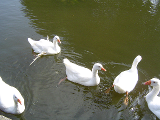 |
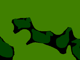 |
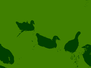 |
In the densecrf reference annotation, pure black (0, 0, 0) marks pixels
where no class is asserted; every other unique RGB triplet is one class.
The unary follows the densecrf convention: labeled pixels get the
assigned class with probability gt_prob = 0.7 and split the remaining
mass equally; black ("unknown") pixels get a uniform prior. Mean-field
then propagates labels into the unknown regions guided by image edges.
Going higher: 7D trilateral CRF¶
The 5D bilateral CRF generalizes to RGB video by adding a time axis to position. Choy, Gwak, & Savarese (CVPR 2019) ("4D Spatio-Temporal ConvNets: Minkowski Convolutional Neural Networks") introduce a trilateral-stationary CRF for 4D video segmentation in their §5: lift each voxel into
and run the same mean-field algorithm with sparse convolution on the 7D lattice. The dense version of this would touch \(\gtrsim 10^{15}\) cells; only the occupied voxels matter, so the sparse-convolution machinery is not just an optimization but the only tractable path. The compatibility matrix \(\mu\) is learned (1×1 conv across labels), and the kernel and weights are trained jointly with the backbone — i.e., the entire CRF is a differentiable head.
The 2D example here is the same algorithm at \(d = 5\) instead of \(d = 7\), with Potts compatibility instead of a learned \(\mu\). The pattern transfers: the higher the dimension, the more sparse convolution earns its keep.
References¶
- Krähenbühl, Koltun. Efficient Inference in Fully Connected CRFs with Gaussian Edge Potentials. NeurIPS 2011. arXiv:1210.5644.
- Adams, Baek, Davis. Fast High-Dimensional Filtering Using the Permutohedral Lattice. Eurographics 2010.
- Zheng et al. Conditional Random Fields as Recurrent Neural Networks. ICCV 2015. arXiv:1502.03240.
- Choy, Gwak, Savarese. 4D Spatio-Temporal ConvNets: Minkowski Convolutional Neural Networks. CVPR 2019, §5 trilateral CRF. arXiv:1904.08755.
- See also Bilateral and Permutohedral Filters for the underlying filter primitives.