Optimization Solvers

cuRobo implements a family of optimization solvers that operate on any class satisfying the Rollout Protocol (see Rollout Classes) to minimize costs and constraints. Every solver accepts a rollout that maps [batch, horizon, dof] actions to [batch, horizon] cost, and every solver itself satisfies the Optimizer Protocol. There is no shared base class – solvers are standalone classes that compose a small set of reusable components.

The solvers fall into three broad categories:

1. Gradient-based solvers (curobo._src.optim.gradient) – use the rollout’s gradient to take Newton-ish steps with a parallel line search.

2. Particle-based solvers (curobo._src.optim.particle) – sample actions from a Gaussian distribution and update the distribution from the cost statistics.

3. External solvers (curobo._src.optim.external) – delegate the outer loop to ScipyOpt (SciPy) or TorchOpt (torch.optim) while still evaluating costs and gradients on the GPU through the cuRobo rollout.

Multiple solvers can be chained into a single solve via MultiStageOptimizer, which itself implements the Optimizer Protocol (see Chaining Optimization Solvers below).

Optimizer Protocol and the composition of its concrete implementations

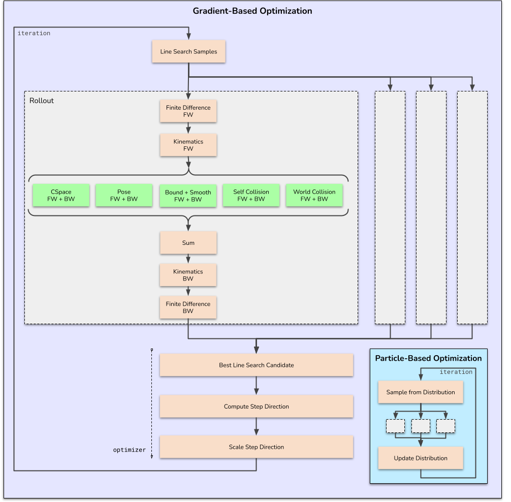
Gradient-Based Optimization Solvers

The gradient-based solvers that cuRobo implements use a parallel line search strategy on the GPU to find the minimum instead of a sequential line search strategy (e.g., backtracking line search). At every iteration of a line-search based optimization solver, cuRobo performs the following steps:

1. Compute the cost and gradient of the current action.

2. Compute a step direction based on the gradient (and possibly other information).

3. Perform a line search to find the best step size along the step direction.

4. Update the action using the step direction and step size.

5. Repeat until convergence or maximum iterations reached.

The specific implementation details vary depending on the optimization algorithm being used (LBFGS, CG, etc.).

Line Search Optimization

1. Compute the best step magnitude using line search from the current action and step direction (from previous iteration).

2. Store the best action and gradient.

3. Compute the new step direction using the gradient of the best action.

Line Search Optimization Iteration

Particle-Based Optimization Solvers

Particle-based solvers sample a batch of candidate actions from a Gaussian distribution over the action sequence, score each sample with the rollout, and update the distribution from the cost-weighted statistics. cuRobo ships two particle solvers:

• MPPI – Model-Predictive Path Integral control. Computes exponential-utility weights (w ∝ exp(-beta * cost)) and takes an exponentially-moving-average step on the distribution mean and covariance. The beta temperature is the primary tuning knob for the exploration/exploitation trade-off.

• EvolutionStrategies – a natural- gradient evolution-strategies solver that uses z-score-normalised cost weights and a configurable learning_rate for the mean update.

Both solvers share the same hot loop: they compose a ParticleOptCore, which owns the GaussianDistribution, ActionBounds, and DebugRecorder, and drives sampling, rollout evaluation, and weight computation. The solvers differ only in their distribution-update function; everything else is reused through composition.

External Optimization Solvers

External solvers delegate the optimizer loop to a third-party library while still evaluating costs, constraints, and gradients on the GPU through the cuRobo rollout. Both external solvers compose ActionBounds (for projecting and scaling actions) and DebugRecorder (for optional per-iteration traces).

Scipy Optimization

The ScipyOpt solver wraps scipy.optimize.minimize. On each iteration it:

1. Computes costs, constraints, and gradients on the GPU via the rollout.

2. Transfers the scalar cost and gradient to CPU.

3. Hands control to SciPy (e.g. L-BFGS-B or SLSQP) to produce the next action.

The method is selected through scipy_minimize_method on ScipyOptCfg. Constraint-aware methods like SLSQP automatically receive cuRobo constraints as inequality constraints, and the action is converted to float64 on CPU for numerical stability.

Torch Optimization

The TorchOpt solver wraps any optimizer from torch.optim (e.g. Adam, SGD, LBFGS). It computes the cost via the rollout, backpropagates through the computation graph, and delegates the parameter update to the wrapped PyTorch optimizer. The specific optimizer class is selected by torch_optim_name (looked up in torch.optim) or by passing an explicit torch_optim_class. Unlike the gradient-based solvers above, TorchOpt does not use cuRobo’s parallel line search – the wrapped PyTorch optimizer owns the step-size logic.

Chaining Optimization Solvers

cuRobo chains solvers through MultiStageOptimizer, which itself satisfies the Optimizer Protocol. Each stage runs to completion and its output is fed as the seed for the next. This is how curobo.inverse_kinematics.InverseKinematics and curobo.trajectory_optimizer.TrajectoryOptimizer are wired: a random seed is first optimized by MPPI for global exploration, and the resulting distribution mean is handed to LBFGSOpt for local refinement.

The steps inside the optimization solver is illustrated for reference. Gray blocks indicate running rollout for 1 trajectory in the batch and green blocks refer to the cost terms.