plot_angular_scan#
- sionna.phy.isac.plot_angular_scan(angular_spectrum: torch.Tensor, theta: torch.Tensor, phi: torch.Tensor, *, display_unit: Literal['rad', 'deg'] = 'deg', scale: Literal['linear', 'db'] = 'db', normalize: bool = True, db_floor: float = -40.0, ax: matplotlib.axes._axes.Axes | None = None, cmap: str = 'viridis') Tuple[matplotlib.figure.Figure, matplotlib.axes._axes.Axes][source]#
Plot a selected theta-phi angular spectrum.
The map value at indices \((i,j)\) is displayed at zenith and azimuth coordinates \((\theta_i,\varphi_j)\). Both are always provided in radians and can be converted to degrees for display.
- Parameters:
angular_spectrum (torch.Tensor) – Selected linear-power angular spectrum with shape [num_theta, num_phi].
theta (torch.Tensor) – Zenith coordinates [rad], shape [num_theta].
phi (torch.Tensor) – Azimuth coordinates [rad], shape [num_phi].
display_unit (Literal['rad', 'deg']) – Unit used for displaying
thetaandphi,"rad"or"deg". Defaults to"deg".scale (Literal['linear', 'db']) – Power-display scale,
"linear"or"db". Defaults to"db".normalize (bool) – If True, normalize the displayed spectrum by its maximum. Defaults to True.
db_floor (float) – Smallest displayed value in decibels. Only used for
scale="db". Defaults to -40.ax (matplotlib.axes._axes.Axes | None) – Matplotlib axes into which the spectrum is drawn. If None, a new figure and axes are created.
cmap (str) – Matplotlib colormap.
- Outputs:
fig – matplotlib.figure.Figure. Figure containing the plot.
ax – matplotlib.axes.Axes. Axes containing the plot.
Examples
The following example plots a synthetic theta-phi spectrum.
import matplotlib.pyplot as plt
import torch
from sionna.phy.isac import plot_angular_scan

theta = torch.deg2rad(torch.linspace(60., 120., 31))
phi = torch.deg2rad(torch.linspace(-60., 60., 61))
angular_spectrum = torch.exp(
    -((theta[:, None]-1.41)/0.15)**2
    -((phi[None, :]-0.33)/0.2)**2)
fig, ax = plot_angular_scan(angular_spectrum, theta, phi)
plt.show()
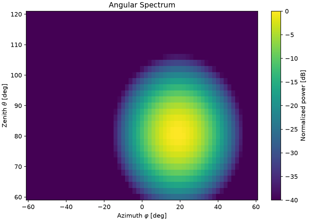
Fig. 26 Synthetic theta-phi angular spectrum.#