plot_delay_doppler#
- sionna.phy.isac.plot_delay_doppler(delay_doppler_spectrum: torch.Tensor, *, l_min: int = 0, fast_time_sample_rate: float | None = None, slow_time_sample_rate: float | None = None, wavelength: float | None = None, domain: Literal['auto', 'index', 'delay_doppler', 'range_velocity'] = 'auto', scale: Literal['linear', 'db'] = 'db', normalize: bool = True, db_floor: float = -40.0, ax: matplotlib.axes._axes.Axes | None = None, cmap: str = 'viridis') Tuple[matplotlib.figure.Figure, matplotlib.axes._axes.Axes][source]#
Plot a selected delay-Doppler spectrum.
For \(N_\text{D}\) Doppler bins and fast- and slow-time sample rates \(f_\text{fast}\) and \(f_\text{slow}\), the physical coordinates are
\[\begin{split}\tau_\ell &= \frac{\ell}{f_\text{fast}},\\ \nu_q &= \frac{q f_\text{slow}}{N_\text{D}},\end{split}\]where \(\ell=L_\text{min},\ldots,L_\text{min}+N_\text{L}-1\) for \(N_\text{L}\) delay bins and \(q=-\lfloor N_\text{D}/2\rfloor,\ldots, N_\text{D}-\lfloor N_\text{D}/2\rfloor-1\). For monostatic sensing, these coordinates can be converted to range and radial velocity according to
\[R_\ell = \frac{c\tau_\ell}{2}, \qquad v_q = \frac{\lambda\nu_q}{2}.\]A positive Doppler frequency, and hence a positive radial velocity, corresponds to a target moving towards the sensing device.
Delays and Doppler frequencies are displayed in microseconds and kilohertz, ranges and radial velocities in meters and meters per second.
- Parameters:
delay_doppler_spectrum (torch.Tensor) – Selected linear-power spectrum with shape [num_doppler_bins, num_delay_bins]. Doppler bins must use centered ordering.
l_min (int) – Time lag of the first delay bin (\(L_\text{min}\)). Must match the
l_minpassed toofdm_to_delay_doppler_channel(). Defaults to 0.fast_time_sample_rate (float | None) – Fast-time sample rate [Hz]. Required for physical delay, range, Doppler, or velocity axes. Must be finite and strictly positive.
slow_time_sample_rate (float | None) – Slow-time sample rate [Hz]. Required for physical delay, range, Doppler, or velocity axes. Must be finite and strictly positive.
wavelength (float | None) – Carrier wavelength [m]. Must be finite and strictly positive. Required when
domain="range_velocity"and ignored otherwise.domain (Literal['auto', 'index', 'delay_doppler', 'range_velocity']) – Axis domain.
"auto"uses indices if both sample rates are omitted and delay/Doppler otherwise."index"always uses bin indices. Defaults to"auto".scale (Literal['linear', 'db']) – Power-display scale,
"linear"or"db". Defaults to"db".normalize (bool) – If True, normalize the displayed spectrum by its maximum. Defaults to True.
db_floor (float) – Smallest displayed value in decibels. Only used for
scale="db". Defaults to -40.ax (matplotlib.axes._axes.Axes | None) – Matplotlib axes into which the spectrum is drawn. If None, a new figure and axes are created.
cmap (str) – Matplotlib colormap.
- Outputs:
fig – matplotlib.figure.Figure. Figure containing the plot.
ax – matplotlib.axes.Axes. Axes containing the plot.
Examples
The following example plots a synthetic off-grid delay-Doppler spectrum.
import matplotlib.pyplot as plt
import torch
from sionna.phy.isac import plot_delay_doppler

delay = torch.arange(64)
doppler = torch.arange(-16, 16)
delay_doppler_spectrum = (
    torch.sinc(doppler[:, None]-2.35).square()
    * torch.sinc(delay[None, :]-10.4).square())
fig, ax = plot_delay_doppler(delay_doppler_spectrum)
plt.show()
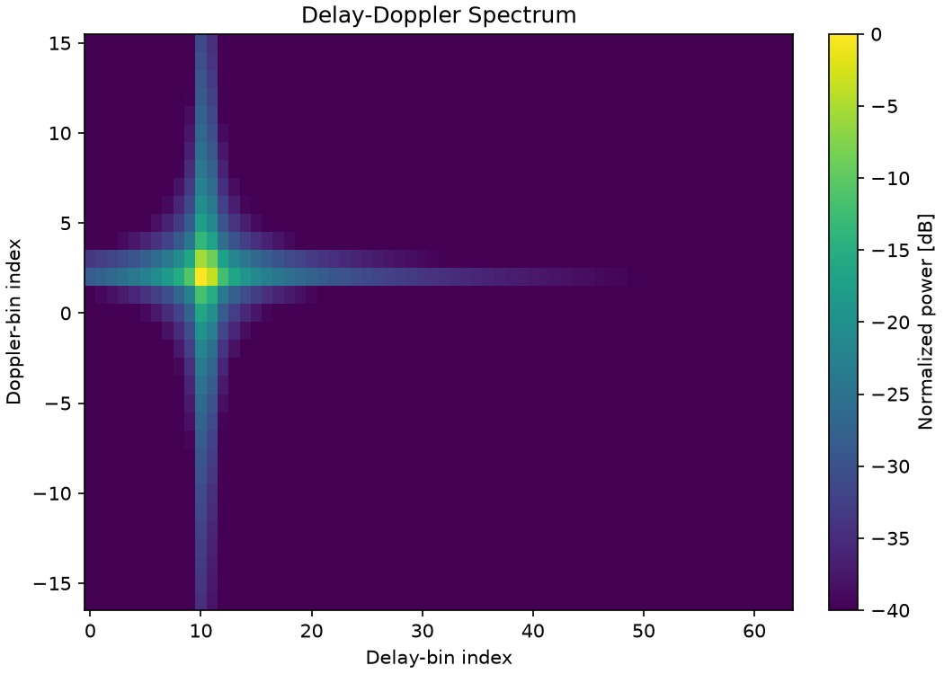
Fig. 27 Synthetic off-grid delay-Doppler spectrum.#