ofdm_to_time_channel#
- sionna.phy.channel.ofdm_to_time_channel(h_f: torch.Tensor, l_min: int = 0, l_max: int | None = None) torch.Tensor[source]#
Compute the discrete complex-baseband channel impulse response from a channel frequency response on a complete OFDM frequency grid
Given a channel frequency response \(\hat{h}_{b,n}\), the channel taps are computed as
\[\bar{h}_{b,\ell} = \frac{1}{N}\sum_{n=0}^{N-1} \hat{h}_{b,n}e^{j\frac{2\pi n\ell}{N}},\]for \(\ell=L_\text{min},\ldots,L_\text{max}\), where \(N\) is
fft_size, \(b\) is the time-step index, \(n\) is the frequency-bin index after undoing the centered subcarrier ordering, and \(\ell\) is the time-lag index. Ifl_maxis None, \(L_\text{max}=L_\text{min}+N-1\).- Parameters:
h_f (torch.Tensor) – Channel frequency responses on a complete, uniformly spaced OFDM frequency grid in centered subcarrier order, shape […, num_time_steps, fft_size]
l_min (int) – Smallest time-lag for the discrete complex-baseband channel impulse response (\(L_{\text{min}}\)). Defaults to 0.
l_max (int | None) – Largest time-lag for the discrete complex-baseband channel impulse response (\(L_{\text{max}}\)). If None, all
fft_sizelags starting atl_minare returned. Defaults to None.
- Outputs:
h_t – […, num_time_steps, num_time_lags], torch.complex. Channel taps ordered from
l_mintol_max. Ifl_maxis None,num_time_lags = fft_size; otherwise,num_time_lags = l_max-l_min+1.
Notes
The last dimension of
h_fmust use the centered subcarrier ordering produced bytime_to_ofdm_channel(). The inverse DFT represents time lags circularly modulofft_size; negative lags are reordered according tol_minbefore the requested interval is selected. With the default arguments, the canonical circular lags from 0 tofft_size-1are returned. As lags are only determined modulofft_size,l_minmust satisfy-fft_size < l_min < fft_size.Due to the \(1/N\) normalization, a path with a delay on the sampling grid appears as a single tap equal to its path coefficient, and the channel energy is preserved, \(\sum_{\ell}|\bar{h}_{b,\ell}|^2 = \frac{1}{N}\sum_{n=0}^{N-1}|\hat{h}_{b,n}|^2\), if all
fft_sizelags are returned. Selecting fewer lags can only reduce the energy.This function inverts the Fourier transform and lag reordering performed by
time_to_ofdm_channel(), but it cannot reconstruct channel samples discarded by that function’s temporal downsampling. The input must contain a complete, uniformly spaced DFT grid; selected or irregularly spaced subcarriers are insufficient.Applying this function to the output of
cir_to_ofdm_channel()is generally different from callingcir_to_time_channel()on the same channel impulse response. The latter samples a sinc response, whereas this function computes the periodic inverse DFT of a finite frequency grid. Both representations coincide for path delays aligned with the sampling grid, but generally differ for fractional delays.Examples
import matplotlib.pyplot as plt
import torch
from sionna.phy import config
from sionna.phy.channel import (cir_to_ofdm_channel,
    cir_to_time_channel, ofdm_to_time_channel,
    subcarrier_frequencies, time_lag_discrete_time_channel)
from sionna.phy.channel.tr38901 import TDL
from sionna.phy.ofdm import ResourceGrid

# Setup resource grid and channel model
config.seed = 42
rg = ResourceGrid(num_ofdm_symbols=1,
                  fft_size=64,
                  subcarrier_spacing=240e3)
tdl = TDL("A", 100e-9, 3.5e9)

# Generate CIR and select the time-lag interval
cir = tdl(batch_size=1, num_time_steps=1,
          sampling_frequency=rg.bandwidth)
l_min, l_max = time_lag_discrete_time_channel(rg.bandwidth)

# Convert the CIR directly to a time channel
h_t = cir_to_time_channel(rg.bandwidth, *cir,
                          l_min=l_min, l_max=l_max).squeeze()

# Convert the CIR through the OFDM representation
frequencies = subcarrier_frequencies(rg.fft_size,
                                     rg.subcarrier_spacing)
h_f = cir_to_ofdm_channel(frequencies, *cir).squeeze()
h_t_from_ofdm = ofdm_to_time_channel(h_f, l_min, l_max).squeeze()

# Compare the two time-channel representations
lags = torch.arange(l_min, l_max + 1)
error = (h_t - h_t_from_ofdm).abs().cpu()
fig, axes = plt.subplots(2, 1, figsize=(7, 6), sharex=True,
                         height_ratios=[2, 1])
axes[0].plot(lags, h_t.abs().cpu(), "o-", markersize=3,
             label="Sampled sinc response")
axes[0].plot(lags, h_t_from_ofdm.abs().cpu(), "x--", markersize=4,
             label="Finite-grid inverse DFT")
axes[0].set_ylabel("Channel magnitude")
axes[0].grid()
axes[0].legend()
axes[1].semilogy(lags, error, "o-", markersize=3)
axes[1].set_xlabel("Time lag")
axes[1].set_ylabel("Absolute difference")
axes[1].grid()
plt.show()
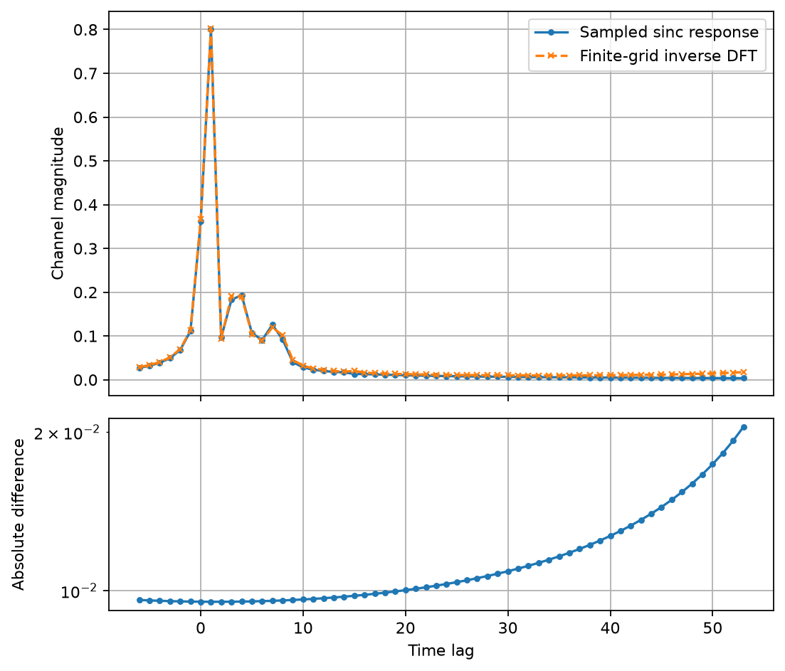
Fig. 22 Comparison of the sampled sinc response and the periodic inverse DFT of the corresponding finite OFDM frequency grid.#