Utility Functions

This module provides utility functions for the FEC package. It also provides serval functions to simplify EXIT analysis of iterative receivers.

(Binary) Linear Codes

Several functions are provided to convert parity-check matrices into generator matrices and vice versa. Please note that currently only binary codes are supported.

# load example parity-check matrix
pcm, k, n, coderate = load_parity_check_examples(pcm_id=3)

Note that many research projects provide their parity-check matrices in the alist format [MacKay] (e.g., see [UniKL]). The follwing code snippet provides an example of how to import an external LDPC parity-check matrix from an alist file and how to set-up an encoder/decoder.

# load external example parity-check matrix in alist format
al = load_alist(path=filename)
pcm, k, n, coderate = alist2mat(al)

# the linear encoder can be directly initialized with a parity-check matrix
encoder = LinearEncoder(pcm, is_pcm=True)

# initalize BP decoder for the given parity-check matrix
decoder = LDPCBPDecoder(pcm, num_iter=20)

# and run simulation with random information bits
no = 1.
batch_size = 10
num_bits_per_symbol = 2

source = BinarySource()
mapper = Mapper("qam", num_bits_per_symbol)
channel = AWGN()
demapper = Demapper("app", "qam", num_bits_per_symbol)

u = source([batch_size, k])
c = encoder(u)
x = mapper(c)
y = channel([x, no])
llr = demapper([y, no])
c_hat = decoder(llr)

load_parity_check_examples

sionna.fec.utils.load_parity_check_examples(pcm_id, verbose=False)[source]

Utility function to load example codes stored in sub-folder LDPC/codes.

The following codes are available

0 : (7,4)-Hamming code of length k=4 information bits and codeword length n=7.
1 : (63,45)-BCH code of length k=45 information bits and codeword length n=63.
2 : (127,106)-BCH code of length k=106 information bits and codeword length n=127.
3 : Random LDPC code with regular variable node degree 3 and check node degree 6 of length k=50 information bits and codeword length n=100.
4 : 802.11n LDPC code of length of length k=324 information bits and codeword length n=648.

Input

pcm_id (int) – An integer defining which matrix id to load.
verbose (bool) – Defaults to False. If True, the code parameters are printed.

Output

pcm (ndarray of zeros and ones) – An ndarray containing the parity check matrix.
k (int) – An integer defining the number of information bits.
n (int) – An integer defining the number of codeword bits.
coderate (float) – A float defining the coderate (assuming full rank of parity-check matrix).

alist2mat

sionna.fec.utils.alist2mat(alist, verbose=True)[source]

Convert alist [MacKay] code definition to full parity-check matrix.

Many code examples can be found in [UniKL].

About alist (see [MacKay] for details):

1. Row defines parity-check matrix dimension m x n

2. Row defines int with max_CN_degree, max_VN_degree

3. Row defines VN degree of all n column

4. Row defines CN degree of all m rows

Next n rows contain non-zero entries of each column (can be zero padded at the end)

Next m rows contain non-zero entries of each row.

Input

alist (list) – Nested list in alist-format [MacKay].
verbose (bool) – Defaults to True. If True, the code parameters are printed.

Output

(pcm, k, n, coderate) – Tuple:
pcm (ndarray) – NumPy array of shape [n-k, n] containing the parity-check matrix.
k (int) – Number of information bits.
n (int) – Number of codewords bits.
coderate (float) – Coderate of the code.

Note

Use load_alist to import alist from a textfile.

For example, the following code snippet will import an alist from a file called filename:

al = load_alist(path = filename)
pcm, k, n, coderate = alist2mat(al)

load_alist

sionna.fec.utils.load_alist(path)[source]

Read alist-file [MacKay] and return nested list describing the parity-check matrix of a code.

Many code examples can be found in [UniKL].

Input: path (str) – Path to file to be loaded.
Output: alist (list) – A nested list containing the imported alist data.

generate_reg_ldpc

sionna.fec.utils.generate_reg_ldpc(v, c, n, allow_flex_len=True, verbose=True)[source]

Generate random regular (v,c) LDPC codes.

This functions generates a random LDPC parity-check matrix of length n where each variable node (VN) has degree v and each check node (CN) has degree c. Please note that the LDPC code is not optimized to avoid short cycles and the resulting codes may show a non-negligible error-floor. For encoding, the LinearEncoder layer can be used, however, the construction does not guarantee that the pcm has full rank.

Input

v (int) – Desired variable node (VN) degree.
c (int) – Desired check node (CN) degree.
n (int) – Desired codeword length.
allow_flex_len (bool) – Defaults to True. If True, the resulting codeword length can be (slightly) increased.
verbose (bool) – Defaults to True. If True, code parameters are printed.

Output

(pcm, k, n, coderate) – Tuple:
pcm (ndarray) – NumPy array of shape [n-k, n] containing the parity-check matrix.
k (int) – Number of information bits per codeword.
n (int) – Number of codewords bits.
coderate (float) – Coderate of the code.

Note

This algorithm works only for regular node degrees. For state-of-the-art bit-error-rate performance, usually one needs to optimize irregular degree profiles (see [tenBrink]).

make_systematic

sionna.fec.utils.make_systematic(mat, is_pcm=False)[source]

Bring binary matrix in its systematic form.

Input

mat (ndarray) – Binary matrix to be transformed to systematic form of shape [k, n].
is_pcm (bool) – Defaults to False. If true, mat is interpreted as parity-check matrix and, thus, the last k columns will be the identity part.

Output

mat_sys (ndarray) – Binary matrix in systematic form, i.e., the first k columns equal the identity matrix (or last k if is_pcm is True).
column_swaps (list of int tuples) – A list of integer tuples that describes the swapped columns (in the order of execution).

Note

This algorithm (potentially) swaps columns of the input matrix. Thus, the resulting systematic matrix (potentially) relates to a permuted version of the code, this is defined by the returned list column_swap. Note that, the inverse permutation must be applied in the inverse list order (in case specific columns are swapped multiple times).

If a parity-check matrix is passed as input (i.e., is_pcm is True), the identity part will be re-arranged to the last columns.

gm2pcm

sionna.fec.utils.gm2pcm(gm, verify_results=True)[source]

Generate the parity-check matrix for a given generator matrix.

This function brings gm \(\mathbf{G}\) in its systematic form and uses the following relation to find the parity-check matrix \(\mathbf{H}\) in GF(2)

\[\mathbf{G} = [\mathbf{I} | \mathbf{M}] \Leftrightarrow \mathbf{H} = [\mathbf{M} ^t | \mathbf{I}]. \tag{1}\]

This follows from the fact that for an all-zero syndrome, it must hold that

\[\mathbf{H} \mathbf{c}^t = \mathbf{H} * (\mathbf{u} * \mathbf{G})^t = \mathbf{H} * \mathbf{G} ^t * \mathbf{u}^t =: \mathbf{0}\]

where \(\mathbf{c}\) denotes an arbitrary codeword and \(\mathbf{u}\) the corresponding information bits.

This leads to

\[\mathbf{G} * \mathbf{H} ^t =: \mathbf{0}. \tag{2}\]

It can be seen that (1) fulfills (2), as it holds in GF(2) that

\[[\mathbf{I} | \mathbf{M}] * [\mathbf{M} ^t | \mathbf{I}]^t = \mathbf{M} + \mathbf{M} = \mathbf{0}.\]

Input

gm (ndarray) – Binary generator matrix of shape [k, n].
verify_results (bool) – Defaults to True. If True, it is verified that the generated parity-check matrix is orthogonal to the generator matrix in GF(2).

Output

ndarray – Binary parity-check matrix of shape [n-k, n].

Note

This algorithm only works if gm has full rank. Otherwise an error is raised.

pcm2gm

sionna.fec.utils.pcm2gm(pcm, verify_results=True)[source]

Generate the generator matrix for a given parity-check matrix.

This function brings pcm \(\mathbf{H}\) in its systematic form and uses the following relation to find the generator matrix \(\mathbf{G}\) in GF(2)

\[\mathbf{G} = [\mathbf{I} | \mathbf{M}] \Leftrightarrow \mathbf{H} = [\mathbf{M} ^t | \mathbf{I}]. \tag{1}\]

This follows from the fact that for an all-zero syndrome, it must hold that

\[\mathbf{H} \mathbf{c}^t = \mathbf{H} * (\mathbf{u} * \mathbf{G})^t = \mathbf{H} * \mathbf{G} ^t * \mathbf{u}^t =: \mathbf{0}\]

where \(\mathbf{c}\) denotes an arbitrary codeword and \(\mathbf{u}\) the corresponding information bits.

This leads to

\[\mathbf{G} * \mathbf{H} ^t =: \mathbf{0}. \tag{2}\]

It can be seen that (1) fulfills (2) as in GF(2) it holds that

\[[\mathbf{I} | \mathbf{M}] * [\mathbf{M} ^t | \mathbf{I}]^t = \mathbf{M} + \mathbf{M} = \mathbf{0}.\]

Input

pcm (ndarray) – Binary parity-check matrix of shape [n-k, n].
verify_results (bool) – Defaults to True. If True, it is verified that the generated generator matrix is orthogonal to the parity-check matrix in GF(2).

Output

ndarray – Binary generator matrix of shape [k, n].

Note

This algorithm only works if pcm has full rank. Otherwise an error is raised.

verify_gm_pcm

sionna.fec.utils.verify_gm_pcm(gm, pcm)[source]

Verify that generator matrix \(\mathbf{G}\) gm and parity-check matrix \(\mathbf{H}\) pcm are orthogonal in GF(2).

For an all-zero syndrome, it must hold that

\[\mathbf{H} \mathbf{c}^t = \mathbf{H} * (\mathbf{u} * \mathbf{G})^t = \mathbf{H} * \mathbf{G} ^t * \mathbf{u}^t =: \mathbf{0}\]

where \(\mathbf{c}\) denotes an arbitrary codeword and \(\mathbf{u}\) the corresponding information bits.

As \(\mathbf{u}\) can be arbitrary it follows that

\[\mathbf{H} * \mathbf{G} ^t =: \mathbf{0}.\]

Input

gm (ndarray) – Binary generator matrix of shape [k, n].
pcm (ndarray) – Binary parity-check matrix of shape [n-k, n].

Output

bool – True if gm and pcm define a valid pair of parity-check and generator matrices in GF(2).

EXIT Analysis

The LDPC BP decoder allows to track the internal information flow (extrinsic information) during decoding. This can be plotted in so-called EXIT Charts [tenBrinkEXIT] to visualize the decoding convergence.

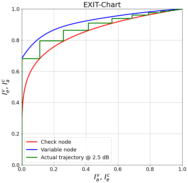
This short code snippet shows how to generate and plot EXIT charts:

# parameters
ebno_db = 2.5 # simulation SNR
batch_size = 10000
num_bits_per_symbol = 2 # QPSK

pcm_id = 4 # decide which parity check matrix should be used (0-2: BCH; 3: (3,6)-LDPC 4: LDPC 802.11n
pcm, k, n , coderate = load_parity_check_examples(pcm_id, verbose=True)

noise_var = ebnodb2no(ebno_db=ebno_db,
                      num_bits_per_symbol=num_bits_per_symbol,
                      coderate=coderate)

# init components
decoder = LDPCBPDecoder(pcm,
                        hard_out=False,
                        cn_type="boxplus",
                        trainable=False,
                        track_exit=True, # if activated, the decoder stores the outgoing extrinsic mutual information per iteration
                        num_iter=20)

# generates fake llrs as if the all-zero codeword was transmitted over an AWNG channel with BPSK modulation
llr_source = GaussianPriorSource()


# generate fake LLRs (Gaussian approximation)
llr = llr_source([[batch_size, n], noise_var])

# simulate free running decoder (for EXIT trajectory)
decoder(llr)

# calculate analytical EXIT characteristics
# Hint: these curves assume asymptotic code length, i.e., may become inaccurate in the short length regime
Ia, Iev, Iec = get_exit_analytic(pcm, ebno_db)

# and plot the analytical exit curves

plt = plot_exit_chart(Ia, Iev, Iec)

# and add simulated trajectory (requires "track_exit=True")
plot_trajectory(plt, decoder.ie_v, decoder.ie_c, ebno_db)

Remark: for rate-matched 5G LDPC codes, the EXIT approximation becomes inaccurate due to the rate-matching and the very specific structure of the code.

plot_exit_chart

sionna.fec.utils.plot_exit_chart(mi_a=None, mi_ev=None, mi_ec=None, title='EXIT-Chart')[source]

Utility function to plot EXIT-Charts [tenBrinkEXIT].

If all inputs are None an empty EXIT chart is generated. Otherwise, the mutual information curves are plotted.

Input

mi_a (float) – An ndarray of floats containing the a priori mutual information.
mi_v (float) – An ndarray of floats containing the variable node mutual information.
mi_c (float) – An ndarray of floats containing the check node mutual information.
title (str) – A string defining the title of the EXIT chart.

Output

plt (matplotlib.figure) – A matplotlib figure handle

Raises

AssertionError – If title is not str.

get_exit_analytic

sionna.fec.utils.get_exit_analytic(pcm, ebno_db)[source]

Calculate the analytic EXIT-curves for a given parity-check matrix.

This function extracts the degree profile from pcm and calculates the variable (VN) and check node (CN) decoder EXIT curves. Please note that this is an asymptotic tool which needs a certain codeword length for accurate predictions.

Transmission over an AWGN channel with BPSK modulation and SNR ebno_db is assumed. The detailed equations can be found in [tenBrink] and [tenBrinkEXIT].

Input

pcm (ndarray) – The parity-check matrix.
ebno_db (float) – The channel SNR in dB.

Output

mi_a (ndarray of floats) – NumPy array containing the a priori mutual information.
mi_ev (ndarray of floats) – NumPy array containing the extrinsic mutual information of the variable node decoder for the corresponding mi_a.
mi_ec (ndarray of floats) – NumPy array containing the extrinsic mutual information of the check node decoder for the corresponding mi_a.

Note

This function assumes random parity-check matrices without any imposed structure. Thus, explicit code construction algorithms may lead to inaccurate EXIT predictions. Further, this function is based on asymptotic properties of the code, i.e., only works well for large parity-check matrices. For details see [tenBrink].

plot_trajectory

sionna.fec.utils.plot_trajectory(plot, mi_v, mi_c, ebno=None)[source]

Utility function to plot the trajectory of an EXIT-chart.

Input

plot (matplotlib.figure) – A handle to a matplotlib figure.
mi_v (float) – An ndarray of floats containing the variable node mutual information.
mi_c (float) – An ndarray of floats containing the check node mutual information.
ebno (float) – A float denoting the EbNo in dB for the legend entry.

Miscellaneous

GaussianPriorSource

class sionna.fec.utils.GaussianPriorSource(specified_by_mi=False, dtype=tf.float32, **kwargs)[source]

Generates fake LLRs as if the all-zero codeword was transmitted over an Bi-AWGN channel with noise variance no or mutual information (if specified_by_mi is True). If selected, the mutual information denotes the mutual information associated with a binary random variable observed at the output of a corresponding AWGN channel (cf. Gaussian approximation).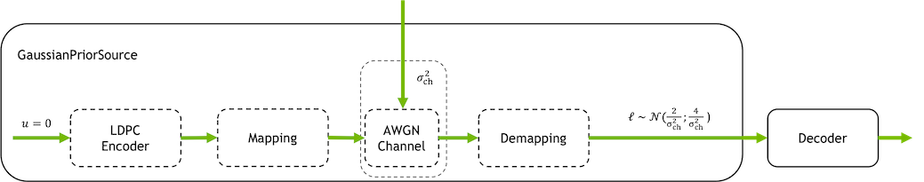

The generated LLRs are drawn from a Gaussian distribution with

\[\sigma_{\text{llr}}^2 = \frac{4}{\sigma_\text{ch}^2}\]

and

\[\mu_{\text{llr}} = \frac{\sigma_\text{llr}^2}{2}\]

where \(\sigma_\text{ch}^2\) is the channel noise variance as defined by no.

If specified_by_mi is True, this class uses the of the so-called J-function (relates mutual information to Gaussian distributed LLRs) as proposed in [Brannstrom].

Parameters

specified_by_mi (bool) – Defaults to False. If True, the second input parameter no is interpreted as mutual information instead of noise variance.
dtype (tf.DType) – Defaults to tf.float32. Defines the datatype for internal calculations and the output. Must be one of the following (tf.float16, tf.bfloat16, tf.float32, tf.float64).

Input

(output_shape, no) – Tuple:
output_shape (tf.int) – Integer tensor or Python array defining the shape of the desired output tensor.
no (tf.float32) – Scalar defining the noise variance or mutual information (if specified_by_mi is True) of the corresponding (fake) AWGN channel.

Output

dtype, defaults to tf.float32 – 1+D Tensor with shape as defined by output_shape.

Raises

InvalidArgumentError – If mutual information is not in (0,1).
AssertionError – If inputs is not a list with 2 elements.

bin2int

sionna.fec.utils.bin2int(arr)[source]

Convert binary array to integer.

For example arr = [1, 0, 1] is converted to 5.

Input: arr (int or float) – An iterable that yields 0’s and 1’s.
Output: int – Integer representation of arr.

int2bin

sionna.fec.utils.int2bin(num, len_)[source]

Convert num of int type to list of length len_ with 0’s and 1’s. num and len_ have to non-negative.

For e.g., num = 5; int2bin(num, len_ =4) = [0, 1, 0, 1].

For e.g., num = 12; int2bin(num, len_ =3) = [1, 0, 0].

Input

num (int) – An integer to be converted into binary representation.
len_ (int) – An integer defining the length of the desired output.

Output

list of int – Binary representation of num of length len_.

bin2int_tf

sionna.fec.utils.bin2int_tf(arr)[source]

Converts binary tensor to int tensor. Binary representation in arr is across the last dimension from most significant to least significant.

For example arr = [0, 1, 1] is converted to 3.

Input: arr (int or float) – Tensor of 0’s and 1’s.
Output: int – Tensor containing the integer representation of arr.

int2bin_tf

sionna.fec.utils.int2bin_tf(ints, len_)[source]

Converts (int) tensor to (int) tensor with 0’s and 1’s. len_ should be to non-negative. Additional dimension of size len_ is inserted at end.

Input

ints (int) – Tensor of arbitrary shape […,k] containing integer to be converted into binary representation.
len_ (int) – An integer defining the length of the desired output.

Output

int – Tensor of same shape as ints except dimension of length len_ is added at the end […,k, len_]. Contains the binary representation of ints of length len_.

int_mod_2

sionna.fec.utils.int_mod_2(x)[source]

Efficient implementation of modulo 2 operation for integer inputs.

This function assumes integer inputs or implicitly casts to int.

Remark: the function tf.math.mod(x, 2) is placed on the CPU and, thus, causes unnecessary memory copies.

Parameters: x (tf.Tensor) – Tensor to which the modulo 2 operation is applied.

llr2mi

sionna.fec.utils.llr2mi(llr, s=None, reduce_dims=True)[source]

Implements an approximation of the mutual information based on LLRs.

The function approximates the mutual information for given llr as derived in [Hagenauer] assuming an all-zero codeword transmission

\[I \approx 1 - \sum \operatorname{log_2} \left( 1 + \operatorname{e}^{-\text{llr}} \right).\]

This approximation assumes that the following symmetry condition is fulfilled

\[p(\text{llr}|x=0) = p(\text{llr}|x=1) \cdot \operatorname{exp}(\text{llr}).\]

For non-all-zero codeword transmissions, this methods requires knowledge about the signs of the original bit sequence s and flips the signs correspondingly (as if the all-zero codeword was transmitted).

Please note that we define LLRs as \(\frac{p(x=1)}{p(x=0)}\), i.e., the sign of the LLRs differ to the solution in [Hagenauer].

Input

llr (tf.float32) – Tensor of arbitrary shape containing LLR-values.
s (None or tf.float32) – Tensor of same shape as llr containing the signs of the transmitted sequence (assuming BPSK), i.e., +/-1 values.
reduce_dims (bool) – Defaults to True. If True, all dimensions are reduced and the return is a scalar. Otherwise, reduce_mean is only taken over the last dimension.

Output

mi (tf.float32) – A scalar tensor (if reduce_dims is True) or a tensor of same shape as llr apart from the last dimensions that is removed. It contains the approximated value of the mutual information.

Raises

TypeError – If dtype of llr is not a real-valued float.

j_fun

sionna.fec.utils.j_fun(mu)[source]

Calculates the J-function in NumPy.

The so-called J-function relates mutual information to the mean of Gaussian distributed LLRs (cf. Gaussian approximation). We use the approximation as proposed in [Brannstrom] which can be written as

\[J(\mu) \approx \left( 1- 2^{H_\text{1}(2\mu)^{H_\text{2}}}\right)^{H_\text{2}}\]

with \(\mu\) denoting the mean value of the LLR distribution and \(H_\text{1}=0.3073\), \(H_\text{2}=0.8935\) and \(H_\text{3}=1.1064\).

Input: mu (float) – float or ndarray of float.
Output: float – ndarray of same shape as the input.

j_fun_inv

sionna.fec.utils.j_fun_inv(mi)[source]

Calculates the inverse J-function in NumPy.

The so-called J-function relates mutual information to the mean of Gaussian distributed LLRs (cf. Gaussian approximation). We use the approximation as proposed in [Brannstrom] which can be written as

\[J(\mu) \approx \left( 1- 2^{H_\text{1}(2\mu)^{H_\text{2}}}\right)^{H_\text{2}}\]

with \(\mu\) denoting the mean value of the LLR distribution and \(H_\text{1}=0.3073\), \(H_\text{2}=0.8935\) and \(H_\text{3}=1.1064\).

Input: mi (float) – float or ndarray of float.
Output: float – ndarray of same shape as the input.
Raises: AssertionError – If mi < 0.001 or mi > 0.999.

j_fun_tf

sionna.fec.utils.j_fun_tf(mu, verify_inputs=True)[source]

Calculates the J-function in Tensorflow.

The so-called J-function relates mutual information to the mean of Gaussian distributed LLRs (cf. Gaussian approximation). We use the approximation as proposed in [Brannstrom] which can be written as

\[J(\mu) \approx \left( 1- 2^{H_\text{1}(2\mu)^{H_\text{2}}}\right)^{H_\text{2}}\]

with \(\mu\) denoting the mean value of the LLR distribution and \(H_\text{1}=0.3073\), \(H_\text{2}=0.8935\) and \(H_\text{3}=1.1064\).

Input

mu (tf.float32) – Tensor of arbitrary shape.
verify_inputs (bool) – A boolean defaults to True. If True, mu is clipped internally to be numerical stable.

Output

tf.float32 – Tensor of same shape and dtype as mu.

Raises

InvalidArgumentError – If mu is negative.

j_fun_inv_tf

sionna.fec.utils.j_fun_inv_tf(mi, verify_inputs=True)[source]

Calculates the inverse J-function in Tensorflow.

The so-called J-function relates mutual information to the mean of Gaussian distributed LLRs (cf. Gaussian approximation). We use the approximation as proposed in [Brannstrom] which can be written as

\[J(\mu) \approx \left( 1- 2^{H_\text{1}(2\mu)^{H_\text{2}}}\right)^{H_\text{2}}\]

with \(\mu\) denoting the mean value of the LLR distribution and \(H_\text{1}=0.3073\), \(H_\text{2}=0.8935\) and \(H_\text{3}=1.1064\).

Input

mi (tf.float32) – Tensor of arbitrary shape.
verify_inputs (bool) – A boolean defaults to True. If True, mi is clipped internally to be numerical stable.

Output

tf.float32 – Tensor of same shape and dtype as the mi.

Raises

InvalidArgumentError – If mi is not in (0,1).

References:

tenBrinkEXIT(1,2,3): S. ten Brink, “Convergence Behavior of Iteratively Decoded Parallel Concatenated Codes,” IEEE Transactions on Communications, vol. 49, no. 10, pp. 1727-1737, 2001.
Brannstrom(1,2,3,4,5): F. Brannstrom, L. K. Rasmussen, and A. J. Grant, “Convergence analysis and optimal scheduling for multiple concatenated codes,” IEEE Trans. Inform. Theory, vol. 51, no. 9, pp. 3354–3364, 2005.
Hagenauer(1,2): J. Hagenauer, “The Turbo Principle in Mobile Communications,” in Proc. IEEE Int. Symp. Inf. Theory and its Appl. (ISITA), 2002.
tenBrink(1,2,3): S. ten Brink, G. Kramer, and A. Ashikhmin, “Design of low-density parity-check codes for modulation and detection,” IEEE Trans. Commun., vol. 52, no. 4, pp. 670–678, Apr. 2004.
MacKay(1,2,3,4,5): http://www.inference.org.uk/mackay/codes/alist.html
UniKL(1,2,3): https://www.uni-kl.de/en/channel-codes/