Basic MIMO Simulations
In this notebook, you will learn how to setup simulations of MIMO transmissions over a flat-fading channel.
Here is a schematic diagram of the system model with all required components:

You will learn how to:
Use the FastFadingChannel class
Apply spatial antenna correlation
Implement LMMSE detection with perfect channel knowledge
Run BER/SER simulations
We will first walk through the configuration of all components of the system model, before building a general Keras model which will allow you to run efficiently simulations with different parameter settings.
Table of Contents
GPU Configuration and Imports
[1]:
import os
if os.getenv("CUDA_VISIBLE_DEVICES") is None:
    gpu_num = 0 # Use "" to use the CPU
    os.environ["CUDA_VISIBLE_DEVICES"] = f"{gpu_num}"
os.environ['TF_CPP_MIN_LOG_LEVEL'] = '3'

# Import Sionna
try:
    import sionna
except ImportError as e:
    # Install Sionna if package is not already installed
    import os
    os.system("pip install sionna")
    import sionna

# Configure the notebook to use only a single GPU and allocate only as much memory as needed
# For more details, see https://www.tensorflow.org/guide/gpu
import tensorflow as tf
gpus = tf.config.list_physical_devices('GPU')
if gpus:
    try:
        tf.config.experimental.set_memory_growth(gpus[0], True)
    except RuntimeError as e:
        print(e)
# Avoid warnings from TensorFlow
tf.get_logger().setLevel('ERROR')

# Set random seed for reproducability
sionna.config.seed = 42
[2]:
%matplotlib inline
import matplotlib.pyplot as plt
import numpy as np
import sys

from sionna.utils import BinarySource, QAMSource, ebnodb2no, compute_ser, compute_ber, PlotBER
from sionna.channel import FlatFadingChannel, KroneckerModel
from sionna.channel.utils import exp_corr_mat
from sionna.mimo import lmmse_equalizer
from sionna.mapping import SymbolDemapper, Mapper, Demapper
from sionna.fec.ldpc.encoding import LDPC5GEncoder
from sionna.fec.ldpc.decoding import LDPC5GDecoder
Simple uncoded transmission
We will consider point-to-point transmissions from a transmitter with num_tx_ant antennas to a receiver with num_rx_ant antennas. The transmitter applies no precoding and sends independent data stream from each antenna.
Let us now generate a batch of random transmit vectors of random 16QAM symbols:
[3]:
num_tx_ant = 4
num_rx_ant = 16
num_bits_per_symbol = 4
batch_size = 1024
qam_source = QAMSource(num_bits_per_symbol)
x = qam_source([batch_size, num_tx_ant])
print(x.shape)
(1024, 4)
Next, we will create an instance of the FlatFadingChannel class to simulate transmissions over an i.i.d. Rayleigh fading channel. The channel will also add AWGN with variance no. As we will need knowledge of the channel realizations for detection, we activate the return_channel flag.
[4]:
channel = FlatFadingChannel(num_tx_ant, num_rx_ant, add_awgn=True, return_channel=True)
no = 0.2 # Noise variance of the channel

# y and h are the channel output and channel realizations, respectively.
y, h = channel([x, no])
print(y.shape)
print(h.shape)
(1024, 16)
(1024, 16, 4)
Using the perfect channel knowledge, we can now implement an LMMSE equalizer to compute soft-symbols. The noise covariance matrix in this example is just a scaled identity matrix which we need to provide to the lmmse_equalizer.
[5]:
s = tf.cast(no*tf.eye(num_rx_ant, num_rx_ant), y.dtype)
x_hat, no_eff = lmmse_equalizer(y, h, s)
Let us know have a look at the transmitted and received constellations:
[6]:
plt.axes().set_aspect(1.0)
plt.scatter(np.real(x_hat), np.imag(x_hat));
plt.scatter(np.real(x), np.imag(x));
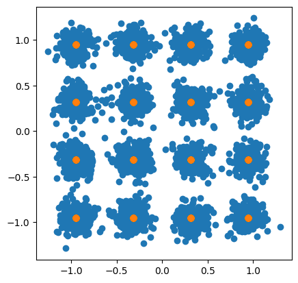
As expected, the soft symbols x_hat are scattered around the 16QAM constellation points. The equalizer output no_eff provides an estimate of the effective noise variance for each soft-symbol.
[7]:
print(no_eff.shape)
(1024, 4)
One can confirm that this estimate is correct by comparing the MSE between the transmitted and equalized symbols against the average estimated effective noise variance:
[8]:
noise_var_eff = np.var(x-x_hat)
noise_var_est = np.mean(no_eff)
print(noise_var_eff)
print(noise_var_est)
0.015844796
0.016486917
The last step is to make hard decisions on the symbols and compute the SER:
[9]:
symbol_demapper = SymbolDemapper("qam", num_bits_per_symbol, hard_out=True)

# Get symbol indices for the transmitted symbols
x_ind = symbol_demapper([x, no])

# Get symbol indices for the received soft-symbols
x_ind_hat = symbol_demapper([x_hat, no])

compute_ser(x_ind, x_ind_hat)
[9]:
<tf.Tensor: shape=(), dtype=float64, numpy=0.00244140625>
Adding spatial correlation
It is very easy add spatial correlation to the FlatFadingChannel using the SpatialCorrelation class. We can, e.g., easily setup a Kronecker (KroneckerModel) (or two-sided) correlation model using exponetial correlation matrices (exp_corr_mat).
[10]:
# Create transmit and receive correlation matrices
r_tx = exp_corr_mat(0.4, num_tx_ant)
r_rx = exp_corr_mat(0.9, num_rx_ant)

# Add the spatial correlation model to the channel
channel.spatial_corr = KroneckerModel(r_tx, r_rx)
Next, we can validate that the channel model applies the desired spatial correlation by creating a large batch of channel realizations from which we compute the empirical transmit and receiver covariance matrices:
[11]:
h = channel.generate(1000000)

# Compute empirical covariance matrices
r_tx_hat = tf.reduce_mean(tf.matmul(h, h, adjoint_a=True), 0)/num_rx_ant
r_rx_hat = tf.reduce_mean(tf.matmul(h, h, adjoint_b=True), 0)/num_tx_ant

# Test that the empirical results match the theory
assert(np.allclose(r_tx, r_tx_hat, atol=1e-2))
assert(np.allclose(r_rx, r_rx_hat, atol=1e-2))
Now, we can transmit the same symbols x over the channel with spatial correlation and compute the SER:
[12]:
y, h = channel([x, no])
x_hat, no_eff = lmmse_equalizer(y, h, s)
x_ind_hat = symbol_demapper([x_hat, no])
compute_ser(x_ind, x_ind_hat)
[12]:
<tf.Tensor: shape=(), dtype=float64, numpy=0.121337890625>
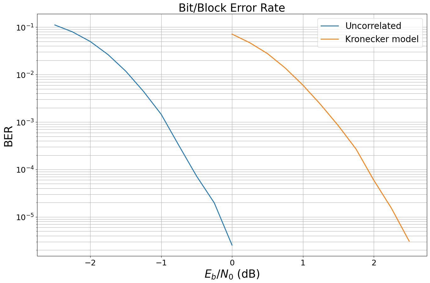
The result cleary show the negative effect of spatial correlation in this setting. You can play around with the a parameter defining the exponential correlation matrices and see its impact on the SER.
Extension to channel coding
So far, we have simulated uncoded symbol transmissions. With a few lines of additional code, we can extend what we have done to coded BER simulations. We need the following additional components:
[13]:
n = 1024 # codeword length
k = 512  # number of information bits per codeword
coderate = k/n # coderate
batch_size = 32

binary_source = BinarySource()
encoder = LDPC5GEncoder(k, n)
decoder = LDPC5GDecoder(encoder, hard_out=True)
mapper = Mapper("qam", num_bits_per_symbol)
demapper = Demapper("app", "qam", num_bits_per_symbol)
Next we need to generate random QAM symbols through mapping of coded bits. Reshaping is required to bring x into the needed shape.
[14]:
b = binary_source([batch_size, num_tx_ant, k])
c = encoder(b)
x = mapper(c)
x_ind = symbol_demapper([x, no]) # Get symbol indices for SER computation later on
shape = tf.shape(x)
x = tf.reshape(x, [-1, num_tx_ant])
print(x.shape)
(8192, 4)
We will now transmit the symbols over the channel:
[15]:
y, h = channel([x, no])
x_hat, no_eff = lmmse_equalizer(y, h, s)
And then demap the symbols to LLRs prior to decoding them. Note that we need to bring x_hat and no_eff back to the desired shape for decoding.
[16]:
x_ind_hat.shape
[16]:
TensorShape([1024, 4])
[17]:
x_hat = tf.reshape(x_hat, shape)
no_eff = tf.reshape(no_eff, shape)

llr = demapper([x_hat, no_eff])
b_hat = decoder(llr)

x_ind_hat = symbol_demapper([x_hat, no])
ber = compute_ber(b, b_hat).numpy()
print("Uncoded SER : {}".format(compute_ser(x_ind, x_ind_hat)))
print("Coded BER : {}".format(compute_ber(b, b_hat)))
Uncoded SER : 0.118408203125
Coded BER : 0.0
Despite the fairly high SER, the BER is very low, thanks to the channel code.
BER simulations using a Keras model
Next, we will wrap everything that we have done so far in a Keras model for convenient BER simulations and comparison of model parameters. Note that we use the @tf.function(jit_compile=True) decorator which will speed-up the simulations tremendously. See https://www.tensorflow.org/guide/function for further information. You need to enable the sionna.config.xla_compat feature prior to executing the model.
[18]:
sionna.config.xla_compat=True
class Model(tf.keras.Model):
    def __init__(self, spatial_corr=None):
        super().__init__()
        self.n = 1024
        self.k = 512
        self.coderate = self.k/self.n
        self.num_bits_per_symbol = 4
        self.num_tx_ant = 4
        self.num_rx_ant = 16
        self.binary_source = BinarySource()
        self.encoder = LDPC5GEncoder(self.k, self.n)
        self.mapper = Mapper("qam", self.num_bits_per_symbol)
        self.demapper = Demapper("app", "qam", self.num_bits_per_symbol)
        self.decoder = LDPC5GDecoder(self.encoder, hard_out=True)
        self.channel = FlatFadingChannel(self.num_tx_ant,
                                         self.num_rx_ant,
                                         spatial_corr=spatial_corr,
                                         add_awgn=True,
                                         return_channel=True)

    @tf.function(jit_compile=True)
    def call(self, batch_size, ebno_db):
        b = self.binary_source([batch_size, self.num_tx_ant, self.k])
        c = self.encoder(b)

        x = self.mapper(c)
        shape = tf.shape(x)
        x = tf.reshape(x, [-1, self.num_tx_ant])

        no = ebnodb2no(ebno_db, self.num_bits_per_symbol, self.coderate)
        no *= np.sqrt(self.num_rx_ant)

        y, h = self.channel([x, no])
        s = tf.complex(no*tf.eye(self.num_rx_ant, self.num_rx_ant), 0.0)

        x_hat, no_eff = lmmse_equalizer(y, h, s)

        x_hat = tf.reshape(x_hat, shape)
        no_eff = tf.reshape(no_eff, shape)

        llr = self.demapper([x_hat, no_eff])
        b_hat = self.decoder(llr)

        return b,  b_hat
XLA can lead to reduced numerical precision. Use with care.
We can now instantiate different version of this model and use the PlotBer class for easy Monte-Carlo simulations.
[19]:
ber_plot = PlotBER()
[20]:
model1 = Model()

ber_plot.simulate(model1,
        np.arange(-2.5, 0.25, 0.25),
        batch_size=4096,
        max_mc_iter=1000,
        num_target_block_errors=100,
        legend="Uncorrelated",
        show_fig=False);
WARNING: All log messages before absl::InitializeLog() is called are written to STDERR
I0000 00:00:1727354098.000157  220681 device_compiler.h:186] Compiled cluster using XLA!  This line is logged at most once for the lifetime of the process.
EbNo [dB] |        BER |       BLER |  bit errors |    num bits | block errors |  num blocks | runtime [s] |    status
---------------------------------------------------------------------------------------------------------------------------------------
     -2.5 | 1.1128e-01 | 9.2206e-01 |      933516 |     8388608 |        15107 |       16384 |         7.8 |reached target block errors
    -2.25 | 7.9466e-02 | 7.8345e-01 |      666612 |     8388608 |        12836 |       16384 |         0.3 |reached target block errors
     -2.0 | 4.9899e-02 | 5.8502e-01 |      418585 |     8388608 |         9585 |       16384 |         0.3 |reached target block errors
    -1.75 | 2.6456e-02 | 3.6597e-01 |      221930 |     8388608 |         5996 |       16384 |         0.2 |reached target block errors
     -1.5 | 1.1851e-02 | 1.9061e-01 |       99411 |     8388608 |         3123 |       16384 |         0.3 |reached target block errors
    -1.25 | 4.4475e-03 | 8.2764e-02 |       37308 |     8388608 |         1356 |       16384 |         0.3 |reached target block errors
     -1.0 | 1.4606e-03 | 2.8503e-02 |       12252 |     8388608 |          467 |       16384 |         0.2 |reached target block errors
    -0.75 | 3.2067e-04 | 7.3853e-03 |        2690 |     8388608 |          121 |       16384 |         0.2 |reached target block errors
     -0.5 | 7.2420e-05 | 2.1210e-03 |        2430 |    33554432 |          139 |       65536 |         1.0 |reached target block errors
    -0.25 | 1.9709e-05 | 4.3945e-04 |        2480 |   125829120 |          108 |      245760 |         3.8 |reached target block errors
      0.0 | 2.5459e-06 | 7.0155e-05 |        1858 |   729808896 |          100 |     1425408 |        21.9 |reached target block errors
[21]:
r_tx = exp_corr_mat(0.4, num_tx_ant)
r_rx = exp_corr_mat(0.7, num_rx_ant)
model2 = Model(KroneckerModel(r_tx, r_rx))

ber_plot.simulate(model2,
        np.arange(0,2.6,0.25),
        batch_size=4096,
        max_mc_iter=1000,
        num_target_block_errors=200,
        legend="Kronecker model");
EbNo [dB] |        BER |       BLER |  bit errors |    num bits | block errors |  num blocks | runtime [s] |    status
---------------------------------------------------------------------------------------------------------------------------------------
      0.0 | 7.1577e-02 | 7.1643e-01 |      600435 |     8388608 |        11738 |       16384 |         5.3 |reached target block errors
     0.25 | 4.7079e-02 | 5.3833e-01 |      394928 |     8388608 |         8820 |       16384 |         0.3 |reached target block errors
      0.5 | 2.7786e-02 | 3.5327e-01 |      233090 |     8388608 |         5788 |       16384 |         0.3 |reached target block errors
     0.75 | 1.3830e-02 | 1.9855e-01 |      116011 |     8388608 |         3253 |       16384 |         0.3 |reached target block errors
      1.0 | 6.0138e-03 | 9.7351e-02 |       50447 |     8388608 |         1595 |       16384 |         0.3 |reached target block errors
     1.25 | 2.3426e-03 | 4.3274e-02 |       19651 |     8388608 |          709 |       16384 |         0.3 |reached target block errors
      1.5 | 8.3852e-04 | 1.5869e-02 |        7034 |     8388608 |          260 |       16384 |         0.3 |reached target block errors
     1.75 | 2.6973e-04 | 4.7404e-03 |        6788 |    25165824 |          233 |       49152 |         0.8 |reached target block errors
      2.0 | 5.9626e-05 | 1.2096e-03 |        5502 |    92274688 |          218 |      180224 |         3.0 |reached target block errors
     2.25 | 1.5199e-05 | 3.2445e-04 |        4845 |   318767104 |          202 |      622592 |        10.1 |reached target block errors
      2.5 | 3.0807e-06 | 6.4231e-05 |        4936 |  1602224128 |          201 |     3129344 |        50.9 |reached target block errors