Ray Tracing

This module provides a differentiable ray tracer for radio propagation modeling. The best way to get started is by having a look at the Sionna Ray Tracing Tutorial. The Primer on Electromagnetics provides useful background knowledge and various definitions that are used throughout the API documentation.

The most important component of the ray tracer is the Scene. It has methods for the computation of propagation Paths (compute_paths()) and CoverageMap (coverage_map()). Sionna has several integrated Example Scenes that you can use for your own experiments. In this video, we explain how you can create your own scenes using OpenStreetMap and Blender. You can preview a scene within a Jupyter notebook (preview()) or render it to a file from the viewpoint of a camera (render() or render_to_file()).

Propagation Paths can be transformed into time-varying channel impulse responses (CIRs) via cir(). The CIRs can then be used for link-level simulations in Sionna via the functions cir_to_time_channel() or cir_to_ofdm_channel(). Alternatively, you can create a dataset of CIRs that can be used by a channel model with the help of CIRDataset.

The paper Sionna RT: Differentiable Ray Tracing for Radio Propagation Modeling shows how differentiable ray tracing can be used for various optimization tasks. The related notebooks can be a good starting point for your own experiments.

Scene

The scene contains everything that is needed for radio propagation simulation and rendering.

A scene is a collection of multiple instances of SceneObject which define the geometry and materials of the objects in the scene. The scene also includes transmitters (Transmitter) and receivers (Receiver) for which propagation Paths or channel impulse responses (CIRs) can be computed, as well as cameras (Camera) for rendering.

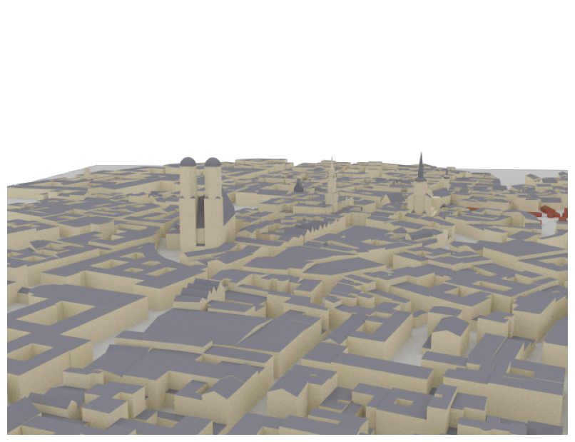
A scene is loaded from a file using the load_scene() function. Sionna contains a few Example Scenes. The following code snippet shows how to load one of them and render it through the lens of the preconfigured scene Camera “scene-cam-0”:

scene = load_scene(sionna.rt.scene.munich)
scene.render(camera="scene-cam-0")

You can preview a scene in an interactive 3D viewer within a Jupyter notebook using preview():

scene.preview()

In the code snippet above, the load_scene() function returns the Scene instance which can be used to access scene objects, transmitters, receivers, cameras, and to set the frequency for radio wave propagation simulation. Note that you can load only a single scene at a time.

It is important to understand that all transmitters in a scene share the same AntennaArray which can be set through the scene property tx_array. The same holds for all receivers whose AntennaArray can be set through rx_array. However, each transmitter and receiver can have a different position and orientation.

The code snippet below shows how to configure the tx_array and rx_array and to instantiate a transmitter and receiver.

# Configure antenna array for all transmitters
scene.tx_array = PlanarArray(num_rows=8,
                          num_cols=2,
                          vertical_spacing=0.7,
                          horizontal_spacing=0.5,
                          pattern="tr38901",
                          polarization="VH")

# Configure antenna array for all receivers
scene.rx_array = PlanarArray(num_rows=1,
                          num_cols=1,
                          vertical_spacing=0.5,
                          horizontal_spacing=0.5,
                          pattern="dipole",
                          polarization="cross")

# Create transmitter
tx = Transmitter(name="tx",
              position=[8.5,21,27],
              orientation=[0,0,0])
scene.add(tx)

# Create a receiver
rx = Receiver(name="rx",
           position=[45,90,1.5],
           orientation=[0,0,0])
scene.add(rx)

# TX points towards RX
tx.look_at(rx)

print(scene.transmitters)
print(scene.receivers)

{'tx': <sionna.rt.transmitter.Transmitter object at 0x7f83d0555d30>}
{'rx': <sionna.rt.receiver.Receiver object at 0x7f81f00ef0a0>}

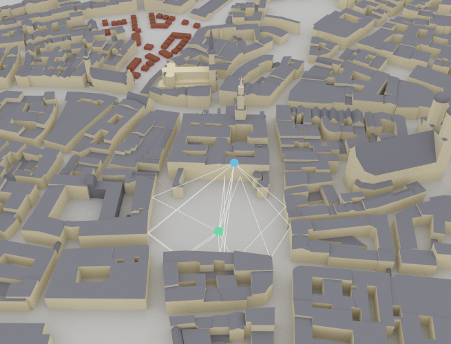
Once you have loaded a scene and configured transmitters and receivers, you can use the scene method compute_paths() to compute propagation paths:

paths = scene.compute_paths()

The output of this function is an instance of Paths and can be used to compute channel impulse responses (CIRs) using the method cir(). You can visualize the paths within a scene by one of the following commands:

scene.preview(paths=paths) # Open preview showing paths
scene.render(camera="preview", paths=paths) # Render scene with paths from preview camera
scene.render_to_file(camera="preview",
                     filename="scene.png",
                     paths=paths) # Render scene with paths to file

Note that the calls to the render functions in the code above use the “preview” camera which is configured through preview(). You can use any other Camera that you create here as well.

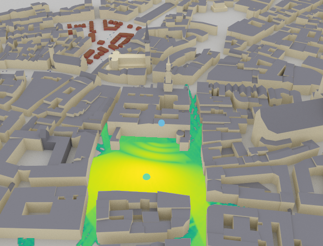
The function coverage_map() computes a CoverageMap for every transmitter in a scene:

cm = scene.coverage_map(cm_cell_size=[1.,1.], # Configure size of each cell
                        num_samples=1e7) # Number of rays to trace

Coverage maps can be visualized in the same way as propagation paths:

scene.preview(coverage_map=cm) # Open preview showing coverage map
scene.render(camera="preview", coverage_map=cm) # Render scene with coverage map
scene.render_to_file(camera="preview",
                     filename="scene.png",
                     coverage_map=cm) # Render scene with coverage map to file

Scene

class sionna.rt.Scene

The scene contains everything that is needed for radio propagation simulation and rendering.

A scene is a collection of multiple instances of SceneObject which define the geometry and materials of the objects in the scene. The scene also includes transmitters (Transmitter) and receivers (Receiver) for which propagation Paths, channel impulse responses (CIRs) or coverage maps (CoverageMap) can be computed, as well as cameras (Camera) for rendering.

The only way to instantiate a scene is by calling load_scene(). Note that only a single scene can be loaded at a time.

Example scenes can be loaded as follows:

scene = load_scene(sionna.rt.scene.munich)
scene.preview()

add(item)

Adds a transmitter, receiver, RIS, radio material, or camera to the scene.

If a different item with the same name as item is already part of the scene, an error is raised.

Input:

item (Transmitter | Receiver | RIS | RadioMaterial | Camera) – Item to add to the scene

property bandwidth

Get/set the transmission bandwidth [Hz]. Used for the computation of thermal_noise_power. Defaults to 1e6.

Type:

float

property cameras

Dictionary of cameras in the scene

Type:

dict (read-only), { “name”, Camera}

property center

Get the center of the scene

Type:

[3], tf.float

property dtype

Datatype used in tensors

Type:

tf.complex64 | tf.complex128

property frequency

Get/set the carrier frequency [Hz]

Setting the frequency updates the parameters of frequency-dependent radio materials. Defaults to 3.5e9.

Type:

float

get(name)

Returns a scene object, transmitter, receiver, camera, or radio material

Input:

name (str) – Name of the item to retrieve

Output:

item (SceneObject | RadioMaterial | Transmitter | Receiver | RIS | Camera | None) – Retrieved item. Returns None if no corresponding item was found in the scene.

property objects

Dictionary of scene objects

Type:

dict (read-only), { “name”, SceneObject}

property radio_material_callable

Get/set a callable that computes the radio material properties at the points of intersection between the rays and the scene objects.

If set, then the RadioMaterial of the objects are not used and the callable is invoked instead to obtain the electromagnetic properties required to simulate the propagation of radio waves.

If not set, i.e., None (default), then the RadioMaterial of objects are used to simulate the propagation of radio waves in the scene.

This callable is invoked on batches of intersection points. It takes as input the following tensors:

• object_id ([batch_dims], int) : Integers uniquely identifying the intersected objects

• points ([batch_dims, 3], float) : Positions of the intersection points

The callable must output a tuple/list of the following tensors:

• complex_relative_permittivity ([batch_dims], complex) : Complex relative permittivities \(\eta\) (9)

• scattering_coefficient ([batch_dims], float) : Scattering coefficients \(S\in[0,1]\) (37)

• xpd_coefficient ([batch_dims], float) : Cross-polarization discrimination coefficients \(K_x\in[0,1]\) (39). Only relevant for the scattered field.

Note: The number of batch dimensions is not necessarily equal to one.

property radio_materials

Dictionary of radio materials

Type:

dict (read-only), { “name”, RadioMaterial}

property receivers

Dictionary of receivers in the scene

Type:

dict (read-only), { “name”, Receiver}

remove(name)

Removes a transmitter, receiver, RIS, camera, or radio material from the scene.

In the case of a radio material, it must not be used by any object of the scene.

Input:

name (str) – Name of the item to remove

property ris

Dictionary of reconfigurable intelligent surfaces (RIS) in the scene

Type:

dict (read-only), { “name”, RIS}

property rx_array

Get/set the antenna array used by all receivers in the scene. Defaults to None.

Type:

AntennaArray

property scattering_pattern_callable

Get/set a callable that computes the scattering pattern at the points of intersection between the rays and the scene objects.

If set, then the scattering_pattern of the radio materials of the objects are not used and the callable is invoked instead to evaluate the scattering pattern required to simulate the propagation of diffusely reflected radio waves.

If not set, i.e., None (default), then the scattering_pattern of the objects’ radio materials are used to simulate the propagation of diffusely reflected radio waves in the scene.

This callable is invoked on batches of intersection points. It takes as input the following tensors:

• object_id ([batch_dims], int) : Integers uniquely identifying the intersected objects

• points ([batch_dims, 3], float) : Positions of the intersection points

• k_i ([batch_dims, 3], float) : Unitary vector corresponding to the direction of incidence in the scene’s global coordinate system

• k_s ([batch_dims, 3], float) : Unitary vector corresponding to the direction of the diffuse reflection in the scene’s global coordinate system

• n ([batch_dims, 3], float) : Unitary vector corresponding to the normal to the surface at the intersection point

The callable must output the following tensor:

• f_s ([batch_dims], float) : The scattering pattern evaluated for the previous inputs

Note: The number of batch dimensions is not necessarily equal to one.

property size

Get the size of the scene, i.e., the size of the axis-aligned minimum bounding box for the scene

Type:

[3], tf.float

property synthetic_array

Get/set if the antenna arrays are applied synthetically. Defaults to True.

Type:

bool

property temperature

Get/set the environment temperature [K]. Used for the computation of thermal_noise_power. Defaults to 293.

Type:

float

property thermal_noise_power

Get the thermal noise power [W]

Type:

float

property transmitters

Dictionary of transmitters in the scene

Type:

dict (read-only), { “name”, Transmitter}

property tx_array

Get/set the antenna array used by all transmitters in the scene. Defaults to None.

Type:

AntennaArray

property wavelength

Get the wavelength [m]

Type:

float (read-only)

property wavenumber

Get the wavenumber \(k=2\pi/\lambda\) [m^-1]

Type:

float (read-only)

compute_paths

sionna.rt.Scene.compute_paths(self, max_depth=3, method='fibonacci', num_samples=1000000, los=True, reflection=True, diffraction=False, scattering=False, ris=True, scat_keep_prob=0.001, edge_diffraction=False, check_scene=True, scat_random_phases=True, testing=False)

Computes propagation paths.

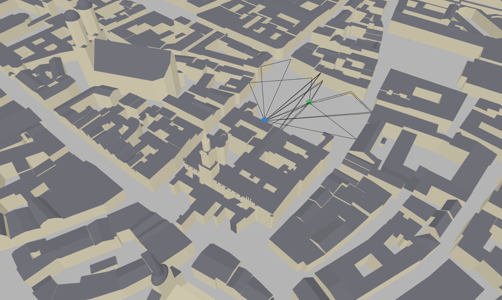
This function computes propagation paths between the antennas of all transmitters and receivers in the current scene. For each propagation path \(i\), the corresponding channel coefficient \(a_i\) and delay \(\tau_i\), as well as the angles of departure \((\theta_{\text{T},i}, \varphi_{\text{T},i})\) and arrival \((\theta_{\text{R},i}, \varphi_{\text{R},i})\) are returned. For more detail, see (26). Different propagation phenomena, such as line-of-sight, reflection, diffraction, and diffuse scattering can be individually enabled/disabled.

If the scene is configured to use synthetic arrays (synthetic_array is True), transmitters and receivers are modelled as if they had a single antenna located at their position. The channel responses for each individual antenna of the arrays are then computed “synthetically” by applying appropriate phase shifts. This reduces the complexity significantly for large arrays. Time evolution of the channel coefficients can be simulated with the help of the function apply_doppler() of the returned Paths object.

The path computation consists of two main steps as shown in the below figure.

For a configured Scene, the function first traces geometric propagation paths using trace_paths(). This step is independent of the RadioMaterial of the scene objects as well as the transmitters’ and receivers’ antenna patterns and orientation, but depends on the selected propagation phenomena, such as reflection, scattering, and diffraction. The traced paths are then converted to EM fields by the function compute_fields(). The resulting Paths object can be used to compute channel impulse responses via cir(). The advantage of separating path tracing and field computation is that one can study the impact of different radio materials by executing compute_fields() multiple times without re-tracing the propagation paths. This can for example speed-up the calibration of scene parameters by several orders of magnitude.

Example

import sionna
from sionna.rt import load_scene, Camera, Transmitter, Receiver, PlanarArray

# Load example scene
scene = load_scene(sionna.rt.scene.munich)

# Configure antenna array for all transmitters
scene.tx_array = PlanarArray(num_rows=8,
                          num_cols=2,
                          vertical_spacing=0.7,
                          horizontal_spacing=0.5,
                          pattern="tr38901",
                          polarization="VH")

# Configure antenna array for all receivers
scene.rx_array = PlanarArray(num_rows=1,
                          num_cols=1,
                          vertical_spacing=0.5,
                          horizontal_spacing=0.5,
                          pattern="dipole",
                          polarization="cross")

# Create transmitter
tx = Transmitter(name="tx",
              position=[8.5,21,27],
              orientation=[0,0,0])
scene.add(tx)

# Create a receiver
rx = Receiver(name="rx",
           position=[45,90,1.5],
           orientation=[0,0,0])
scene.add(rx)

# TX points towards RX
tx.look_at(rx)

# Compute paths
paths = scene.compute_paths()

# Open preview showing paths
scene.preview(paths=paths, resolution=[1000,600])

Input:

• max_depth (int) – Maximum depth (i.e., number of bounces) allowed for tracing the paths. Defaults to 3.

• method (str (“exhaustive”|”fibonacci”)) – Ray tracing method to be used. The “exhaustive” method tests all possible combinations of primitives. This method is not compatible with scattering. The “fibonacci” method uses a shoot-and-bounce approach to find candidate chains of primitives. Initial ray directions are chosen according to a Fibonacci lattice on the unit sphere. This method can be applied to very large scenes. However, there is no guarantee that all possible paths are found. Defaults to “fibonacci”.

• num_samples (int) – Number of rays to trace in order to generate candidates with the “fibonacci” method. This number is split equally among the different transmitters (when using synthetic arrays) or transmit antennas (when not using synthetic arrays). This parameter is ignored when using the exhaustive method. Tracing more rays can lead to better precision at the cost of increased memory requirements. Defaults to 1e6.

• los (bool) – If set to True, then the LoS paths are computed. Defaults to True.

• reflection (bool) – If set to True, then the reflected paths are computed. Defaults to True.

• diffraction (bool) – If set to True, then the diffracted paths are computed. Defaults to False.

• scattering (bool) – If set to True, then the scattered paths are computed. If set to True, then the scattered paths are computed. Only works with the Fibonacci method. Defaults to False.

• ris (bool) – If set to True, then paths involving RIS are computed. Defaults to True.

• scat_keep_prob (float) – Probability with which a scattered path is kept. This is helpful to reduce the number of computed scattered paths, which might be prohibitively high in some scenes. Must be in the range (0,1). Defaults to 0.001.

• edge_diffraction (bool) – If set to False, only diffraction on wedges, i.e., edges that connect two primitives, is considered. Defaults to False.

• check_scene (bool) – If set to True, checks that the scene is well configured before computing the paths. This can add a significant overhead. Defaults to True.

• scat_random_phases (bool) – If set to True and if scattering is enabled, random uniform phase shifts are added to the scattered paths. Defaults to True.

• testing (bool) – If set to True, then additional data is returned for testing. Defaults to False.

Output:

paths : Paths – Simulated paths

trace_paths

sionna.rt.Scene.trace_paths(self, max_depth=3, method='fibonacci', num_samples=1000000, los=True, reflection=True, diffraction=False, scattering=False, ris=True, scat_keep_prob=0.001, edge_diffraction=False, check_scene=True)

Computes the trajectories of the paths by shooting rays.

The EM fields corresponding to the traced paths are not computed. They can be computed using compute_fields():

traced_paths = scene.trace_paths()
paths = scene.compute_fields(*traced_paths)

Path tracing is independent of the radio materials, antenna patterns, and radio device orientations. Therefore, a set of traced paths could be reused for different values of these quantities, e.g., to calibrate the ray tracer. This can enable significant resource savings as path tracing is typically significantly more resource-intensive than field computation.

Note that compute_paths() does both path tracing and field computation.

Input:

• max_depth (int) – Maximum depth (i.e., number of interaction with objects in the scene) allowed for tracing the paths. Defaults to 3.

• method (str (“exhaustive”|”fibonacci”)) – Method to be used to list candidate paths. The “exhaustive” method tests all possible combination of primitives as paths. This method is not compatible with scattering. The “fibonacci” method uses a shoot-and-bounce approach to find candidate chains of primitives. Initial ray directions are arranged in a Fibonacci lattice on the unit sphere. This method can be applied to very large scenes. However, there is no guarantee that all possible paths are found. Defaults to “fibonacci”.

• num_samples (int) – Number of random rays to trace in order to generate candidates. A large sample count may exhaust GPU memory. Defaults to 1e6. Only needed if method is “fibonacci”.

• los (bool) – If set to True, then the LoS paths are computed. Defaults to True.

• reflection (bool) – If set to True, then the reflected paths are computed. Defaults to True.

• diffraction (bool) – If set to True, then the diffracted paths are computed. Defaults to False.

• scattering (bool) – If set to True, then the scattered paths are computed. Only works with the Fibonacci method. Defaults to False.

• ris (bool) – If set to True, then the paths involving RIS are computed. Defaults to True.

• scat_keep_prob (float) – Probability with which to keep scattered paths. This is helpful to reduce the number of scattered paths computed, which might be prohibitively high in some setup. Must be in the range (0,1). Defaults to 0.001.

• edge_diffraction (bool) – If set to False, only diffraction on wedges, i.e., edges that connect two primitives, is considered. Defaults to False.

• check_scene (bool) – If set to True, checks that the scene is well configured before computing the paths. This can add a significant overhead. Defaults to True.

Output:

• spec_paths (Paths) – Computed specular paths

• diff_paths (Paths) – Computed diffracted paths

• scat_paths (Paths) – Computed scattered paths

• ris_paths (Paths) – Computed paths involving RIS

• spec_paths_tmp (PathsTmpData) – Additional data required to compute the EM fields of the specular paths

• diff_paths_tmp (PathsTmpData) – Additional data required to compute the EM fields of the diffracted paths

• scat_paths_tmp (PathsTmpData) – Additional data required to compute the EM fields of the scattered paths

• ris_paths_tmp (PathsTmpData) – Additional data required to compute the EM fields of the paths involving RIS

compute_fields

sionna.rt.Scene.compute_fields(self, spec_paths, diff_paths, scat_paths, spec_paths_tmp, diff_paths_tmp, scat_paths_tmp, check_scene=True, scat_random_phases=True)

Computes the EM fields corresponding to traced paths.

Paths can be traced using trace_paths(). This method can then be used to finalize the paths calculation by computing the corresponding fields:

traced_paths = scene.trace_paths()
paths = scene.compute_fields(*traced_paths)

Paths tracing is independent from the radio materials, antenna patterns, and radio devices orientations. Therefore, a set of traced paths could be reused for different values of these quantities, e.g., to calibrate the ray tracer. This can enable significant resource savings as paths tracing is typically significantly more resource-intensive than field computation.

Note that compute_paths() does both tracing and field computation.

Input:

• spec_paths (Paths) – Specular paths

• diff_paths (Paths) – Diffracted paths

• scat_paths (Paths) – Scattered paths

• ris_paths (Paths) – Computed paths involving RIS

• ris_paths (Paths) – Computed paths involving RIS

• spec_paths_tmp (PathsTmpData) – Additional data required to compute the EM fields of the specular paths

• diff_paths_tmp (PathsTmpData) – Additional data required to compute the EM fields of the diffracted paths

• scat_paths_tmp (PathsTmpData) – Additional data required to compute the EM fields of the scattered paths

• ris_paths_tmp (PathsTmpData) – Additional data required to compute the EM fields of the paths involving RIS

• ris_paths_tmp (PathsTmpData) – Additional data required to compute the EM fields of the paths involving RIS

• check_scene (bool) – If set to True, checks that the scene is well configured before computing the paths. This can add a significant overhead. Defaults to True.

• scat_random_phases (bool) – If set to True and if scattering is enabled, random uniform phase shifts are added to the scattered paths. Defaults to True.

Output:

paths (Paths) – Computed paths

coverage_map

sionna.rt.Scene.coverage_map(self, rx_orientation=(0.0, 0.0, 0.0), max_depth=3, cm_center=None, cm_orientation=None, cm_size=None, cm_cell_size=(10.0, 10.0), combining_vec=None, precoding_vec=None, num_samples=2000000, los=True, reflection=True, diffraction=False, scattering=False, ris=True, edge_diffraction=False, check_scene=True, num_runs=1)

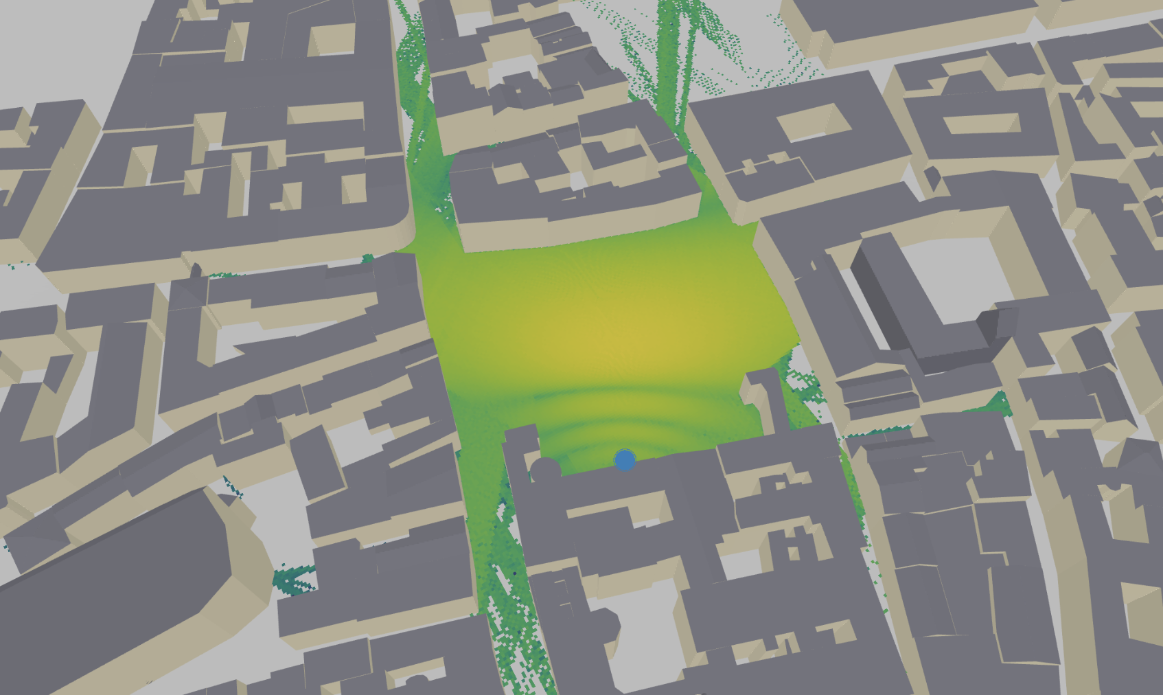
This function computes a coverage map for every transmitter in the scene.

For a given transmitter, a coverage map is a rectangular surface with arbitrary orientation subdivded into rectangular cells of size \(\lvert C \rvert = \texttt{cm_cell_size[0]} \times \texttt{cm_cell_size[1]}\). The parameter cm_cell_size therefore controls the granularity of the map. The coverage map associates with every cell \((i,j)\) the quantity

(52)\[g_{i,j} = \frac{1}{\lvert C \rvert} \int_{C_{i,j}} \lvert h(s) \rvert^2 ds\]

where \(\lvert h(s) \rvert^2\) is the squared amplitude of the path coefficients \(a_i\) at position \(s=(x,y)\), the integral is over the cell \(C_{i,j}\), and \(ds\) is the infinitesimal small surface element \(ds=dx \cdot dy\). The dimension indexed by \(i\) (\(j\)) corresponds to the \(y\, (x)\)-axis of the coverage map in its local coordinate system. The quantity \(g_{i,j}\) can be seen as the average path_gain across a cell.

The path gain can be transformed into the received signal strength (rss) by multiplying it with the transmit power:

\[\mathrm{RSS}_{i,j} = P_{tx} g_{i,j}.\]

If a scene has multiple transmitters, the signal-to-interference-plus-noise ratio (sinr) for transmitter \(k\) is then defined as

\[\mathrm{SINR}^k_{i,j}=\frac{\mathrm{RSS}^k_{i,j}}{N_0+\sum_{k'\ne k} \mathrm{RSS}^{k'}_{i,j}}\]

where \(N_0\) [W] is the thermal_noise_power, computed as:

\[N_0 = B \times T \times k\]

where \(B\) [Hz] is the transmission bandwidth, \(T\) [K] is the temperature, and \(k=1.380649\times 10^{-23}\) [J/K] is the Boltzmann constant.

For specularly and diffusely reflected paths, (52) can be rewritten as an integral over the directions of departure of the rays from the transmitter, by substituting \(s\) with the corresponding direction \(\omega\):

\[g_{i,j} = \frac{1}{\lvert C \rvert} \int_{\Omega} \lvert h\left(s(\omega) \right) \rvert^2 \frac{r(\omega)^2}{\lvert \cos{\alpha(\omega)} \rvert} \mathbb{1}_{\left\{ s(\omega) \in C_{i,j} \right\}} d\omega\]

where the integration is over the unit sphere \(\Omega\), \(r(\omega)\) is the length of the path with direction of departure \(\omega\), \(s(\omega)\) is the point where the path with direction of departure \(\omega\) intersects the coverage map, \(\alpha(\omega)\) is the angle between the coverage map normal and the direction of arrival of the path with direction of departure \(\omega\), and \(\mathbb{1}_{\left\{ s(\omega) \in C_{i,j} \right\}}\) is the function that takes as value one if \(s(\omega) \in C_{i,j}\) and zero otherwise. Note that \(ds = \frac{r(\omega)^2 d\omega}{\lvert \cos{\alpha(\omega)} \rvert}\).

The previous integral is approximated through Monte Carlo sampling by shooting \(N\) rays with directions \(\omega_n\) arranged as a Fibonacci lattice on the unit sphere around the transmitter, and bouncing the rays on the intersected objects until the maximum depth (max_depth) is reached or the ray bounces out of the scene. At every intersection with an object of the scene, a new ray is shot from the intersection which corresponds to either specular reflection or diffuse scattering, following a Bernoulli distribution with parameter the squared scattering coefficient. When diffuse scattering is selected, the direction of the scattered ray is uniformly sampled on the half-sphere. The resulting Monte Carlo estimate is:

(53)\[\hat{g}_{i,j}^{\text{(ref)}} = \frac{4\pi}{N\lvert C \rvert} \sum_{n=1}^N \lvert h\left(s(\omega_n)\right) \rvert^2 \frac{r(\omega_n)^2}{\lvert \cos{\alpha(\omega_n)} \rvert} \mathbb{1}_{\left\{ s(\omega_n) \in C_{i,j} \right\}}.\]

For the diffracted paths, (52) can be rewritten for any wedge with length \(L\) and opening angle \(\Phi\) as an integral over the wedge and its opening angle, by substituting \(s\) with the position on the wedge \(\ell \in [1,L]\) and the angle \(\phi \in [0, \Phi]\):

\[g_{i,j} = \frac{1}{\lvert C \rvert} \int_{\ell} \int_{\phi} \lvert h\left(s(\ell,\phi) \right) \rvert^2 \mathbb{1}_{\left\{ s(\ell,\phi) \in C_{i,j} \right\}} \left\lVert \frac{\partial r}{\partial \ell} \times \frac{\partial r}{\partial \phi} \right\rVert d\ell d\phi\]

where the integral is over the wedge length \(L\) and opening angle \(\Phi\), and \(r\left( \ell, \phi \right)\) is the reparametrization with respected to \((\ell, \phi)\) of the intersection between the diffraction cone at \(\ell\) and the rectangle defining the coverage map (see, e.g., [SurfaceIntegral]). The previous integral is approximated through Monte Carlo sampling by shooting \(N'\) rays from equally spaced locations \(\ell_n\) along the wedge with directions \(\phi_n\) sampled uniformly from \((0, \Phi)\):

(54)\[\hat{g}_{i,j}^{\text{(diff)}} = \frac{L\Phi}{N'\lvert C \rvert} \sum_{n=1}^{N'} \lvert h\left(s(\ell_n,\phi_n)\right) \rvert^2 \mathbb{1}_{\left\{ s(\ell_n,\phi_n) \in C_{i,j} \right\}} \left\lVert \left(\frac{\partial r}{\partial \ell}\right)_n \times \left(\frac{\partial r}{\partial \phi}\right)_n \right\rVert.\]

The output of this function is therefore a real-valued matrix of size [num_cells_y, num_cells_x], for every transmitter, with elements equal to the sum of the contributions of the reflected and scattered paths (53) and diffracted paths (54) for all the wedges, and where

\[\begin{split}\texttt{num_cells_x} = \bigg\lceil\frac{\texttt{cm_size[0]}}{\texttt{cm_cell_size[0]}} \bigg\rceil\\ \texttt{num_cells_y} = \bigg\lceil \frac{\texttt{cm_size[1]}}{\texttt{cm_cell_size[1]}} \bigg\rceil.\end{split}\]

The surface defining the coverage map is a rectangle centered at cm_center, with orientation cm_orientation, and with size cm_size. An orientation of (0,0,0) corresponds to a coverage map parallel to the XY plane, with surface normal pointing towards the \(+z\) axis. By default, the coverage map is parallel to the XY plane, covers all of the scene, and has an elevation of \(z = 1.5\text{m}\). The receiver is assumed to use the antenna array scene.rx_array. If transmitter and/or receiver have multiple antennas, transmit precoding and receive combining are applied which are defined by precoding_vec and combining_vec, respectively.

The \((i,j)\) indices are omitted in the following for clarity. For reflection and scattering, paths are generated by shooting num_samples rays from the transmitters with directions arranged in a Fibonacci lattice on the unit sphere and by simulating their propagation for up to max_depth interactions with scene objects. If max_depth is set to 0 and if los is set to True, only the line-of-sight path is considered. For diffraction, paths are generated by shooting num_samples rays from equally spaced locations along the wedges in line-of-sight with the transmitter, with directions uniformly sampled on the diffraction cone.

For every ray \(n\) intersecting the coverage map cell \((i,j)\), the channel coefficients, \(a_n\), and the angles of departure (AoDs) \((\theta_{\text{T},n}, \varphi_{\text{T},n})\) and arrival (AoAs) \((\theta_{\text{R},n}, \varphi_{\text{R},n})\) are computed. See the Primer on Electromagnetics for more details.

A “synthetic” array is simulated by adding additional phase shifts that depend on the antenna position relative to the position of the transmitter (receiver) as well as the AoDs (AoAs). For the \(k^\text{th}\) transmit antenna and \(\ell^\text{th}\) receive antenna, let us denote by \(\mathbf{d}_{\text{T},k}\) and \(\mathbf{d}_{\text{R},\ell}\) the relative positions (with respect to the positions of the transmitter/receiver) of the pair of antennas for which the channel impulse response shall be computed. These can be accessed through the antenna array’s property positions. Using a plane-wave assumption, the resulting phase shifts from these displacements can be computed as

\[\begin{split}p_{\text{T}, n,k} &= \frac{2\pi}{\lambda}\hat{\mathbf{r}}(\theta_{\text{T},n}, \varphi_{\text{T},n})^\mathsf{T} \mathbf{d}_{\text{T},k}\\ p_{\text{R}, n,\ell} &= \frac{2\pi}{\lambda}\hat{\mathbf{r}}(\theta_{\text{R},n}, \varphi_{\text{R},n})^\mathsf{T} \mathbf{d}_{\text{R},\ell}.\end{split}\]

The final expression for the path coefficient is

\[h_{n,k,\ell} = a_n e^{j(p_{\text{T}, i,k} + p_{\text{R}, i,\ell})}\]

for every transmit antenna \(k\) and receive antenna \(\ell\). These coefficients form the complex-valued channel matrix, \(\mathbf{H}_n\), of size \(\texttt{num_rx_ant} \times \texttt{num_tx_ant}\).

Finally, the coefficient of the equivalent SISO channel is

\[h_n = \mathbf{c}^{\mathsf{H}} \mathbf{H}_n \mathbf{p}\]

where \(\mathbf{c}\) and \(\mathbf{p}\) are the combining and precoding vectors (combining_vec and precoding_vec), respectively.

Example

import sionna
from sionna.rt import load_scene, PlanarArray, Transmitter, Receiver
scene = load_scene(sionna.rt.scene.munich)

# Configure antenna array for all transmitters
scene.tx_array = PlanarArray(num_rows=8,
                        num_cols=2,
                        vertical_spacing=0.7,
                        horizontal_spacing=0.5,
                        pattern="tr38901",
                        polarization="VH")

# Configure antenna array for all receivers
scene.rx_array = PlanarArray(num_rows=1,
                        num_cols=1,
                        vertical_spacing=0.5,
                        horizontal_spacing=0.5,
                        pattern="dipole",
                        polarization="cross")
# Add a transmitters
tx = Transmitter(name="tx",
            position=[8.5,21,30],
            orientation=[0,0,0])
scene.add(tx)
tx.look_at([40,80,1.5])

# Compute coverage map
cm = scene.coverage_map(cm_cell_size=[1.,1.],
                    num_samples=int(10e6))

# Visualize coverage in preview
scene.preview(coverage_map=cm,
            resolution=[1000, 600])

Input:

• rx_orientation ([3], float) – Orientation of the receiver \((\alpha, \beta, \gamma)\) specified through three angles corresponding to a 3D rotation as defined in (3). Defaults to \((0,0,0)\).

• max_depth (int) – Maximum depth (i.e., number of bounces) allowed for tracing the paths. Defaults to 3.

• cm_center ([3], float | None) – Center of the coverage map \((x,y,z)\) as three-dimensional vector. If set to None, the coverage map is centered on the center of the scene, except for the elevation \(z\) that is set to 1.5m. Otherwise, cm_orientation and cm_scale must also not be None. Defaults to None.

• cm_orientation ([3], float | None) – Orientation of the coverage map \((\alpha, \beta, \gamma)\) specified through three angles corresponding to a 3D rotation as defined in (3). An orientation of \((0,0,0)\) or None corresponds to a coverage map that is parallel to the XY plane. If not set to None, then cm_center and cm_scale must also not be None. Defaults to None.

• cm_size ([2], float | None) – Size of the coverage map [m]. If set to None, then the size of the coverage map is set such that it covers the entire scene. Otherwise, cm_center and cm_orientation must also not be None. Defaults to None.

• cm_cell_size ([2], float) – Size of a cell of the coverage map [m]. Defaults to \((10,10)\).

• combining_vec ([num_rx_ant], complex | None) – Combining vector. If set to None, then no combining is applied, and the energy received by all antennas is summed.

• precoding_vec ([num_tx_ant] | [num_tx, num_tx_ant], complex | None) – Precoding vector. If set to None, then defaults to \(\frac{1}{\sqrt{\text{num_tx_ant}}} [1,\dots,1]^{\mathsf{T}}\).

• num_samples (int) – Number of random rays to trace. For the reflected paths, this number is split equally over the different transmitters. For the diffracted paths, it is split over the wedges in line-of-sight with the transmitters such that the number of rays allocated to a wedge is proportional to its length. Defaults to 2e6.

• los (bool) – If set to True, then the LoS paths are computed. Defaults to True.

• reflection (bool) – If set to True, then the reflected paths are computed. Defaults to True.

• diffraction (bool) – If set to True, then the diffracted paths are computed. Defaults to False.

• scattering (bool) – If set to True, then the scattered paths are computed. Defaults to False.

• ris (bool) – If set to True, then paths involving RIS are computed. Defaults to True.

• edge_diffraction (bool) – If set to False, only diffraction on wedges, i.e., edges that connect two primitives, is considered. Defaults to False.

• check_scene (bool) – If set to True, checks that the scene is well configured before computing the coverage map. This can add a significant overhead. Defaults to True.

• num_runs (int, >= 1) – Number of times the coverage map solver is executed. The returned coverage map is the average over all runs. If set to a value greater than one, a random rotation is applied to the Fibonacci lattice at each run. Using mutiple runs can reduce noise in the coverage map without increasing num_samples and the related memory footprint. Defaults to 1.

Output:

cm : CoverageMap – Coverage map

preview

sionna.rt.Scene.preview(self, paths=None, show_paths=True, show_devices=True, show_orientations=False, coverage_map=None, cm_tx=None, cm_db_scale=True, cm_vmin=None, cm_vmax=None, cm_metric='path_gain', resolution=(655, 500), fov=45, background='#ffffff', clip_at=None, clip_plane_orientation=(0, 0, -1))

In an interactive notebook environment, opens an interactive 3D viewer of the scene.

The returned value of this method must be the last line of the cell so that it is displayed. For example:

fig = scene.preview()
# ...
fig

Or simply:

scene.preview()

Default color coding:

• Green: Receiver

• Blue: Transmitter

• Red: Reconfigurable Intelligent Surface (RIS)

Controls:

• Mouse left: Rotate

• Scroll wheel: Zoom

• Mouse right: Move

Input:

• paths (Paths | None) – Simulated paths generated by compute_paths() or None. If None, only the scene is rendered. Defaults to None.

• show_paths (bool) – If paths is not None, shows the paths. Defaults to True.

• show_devices (bool) – If set to True, shows the radio devices. Defaults to True.

• show_orientations (bool) – If show_devices is True, shows the radio devices orientations. Defaults to False.

• coverage_map (CoverageMap | None) – An optional coverage map to overlay in the scene for visualization. Defaults to None.

• cm_tx (int | str | None) – When coverage_map is specified, controls which of the transmitters to display the coverage map for. Either the transmitter’s name or index can be given. If None, the maximum metric over all transmitters is shown. Defaults to None.

• cm_db_scale (bool) – Use logarithmic scale for coverage map visualization, i.e. the coverage values are mapped with: \(y = 10 \cdot \log_{10}(x)\). Defaults to True.

• cm_vmin, cm_vmax (floot | None) – For coverage map visualization, defines the range of path gains that the colormap covers. These parameters should be provided in dB if cm_db_scale is set to True, or in linear scale otherwise. If set to None, then covers the complete range. Defaults to None.

• cm_metric (str, one of [“path_gain”, “rss”, “sinr”]) – Metric of the coverage map to be displayed. Defaults to path_gain.

• resolution ([2], int) – Size of the viewer figure. Defaults to [655, 500].

• fov (float) – Field of view, in degrees. Defaults to 45°.

• background (str) – Background color in hex format prefixed by ‘#’. Defaults to ‘#ffffff’ (white).

• clip_at (float) – If not None, the scene preview will be clipped (cut) by a plane with normal orientation clip_plane_orientation and offset clip_at. That means that everything behind the plane becomes invisible. This allows visualizing the interior of meshes, such as buildings. Defaults to None.

• clip_plane_orientation (tuple[float, float, float]) – Normal vector of the clipping plane. Defaults to (0,0,-1).

render

sionna.rt.Scene.render(self, camera, paths=None, show_paths=True, show_devices=True, coverage_map=None, cm_tx=None, cm_db_scale=True, cm_vmin=None, cm_vmax=None, cm_metric='path_gain', cm_show_color_bar=True, num_samples=512, resolution=(655, 500), fov=45)

Renders the scene from the viewpoint of a camera or the interactive viewer

Input:

• camera (str | Camera) – The name or instance of a Camera. If an interactive viewer was opened with preview(), set to “preview” to use its viewpoint.

• paths (Paths | None) – Simulated paths generated by compute_paths() or None. If None, only the scene is rendered. Defaults to None.

• show_paths (bool) – If paths is not None, shows the paths. Defaults to True.

• show_devices (bool) – If paths is not None, shows the radio devices. Defaults to True.

• coverage_map (CoverageMap | None) – An optional coverage map to overlay in the scene for visualization. Defaults to None.

• cm_tx (int | str | None) – When coverage_map is specified, controls which of the transmitters to display the coverage map for. Either the transmitter’s name or index can be given. If None, the maximum metric over all transmitters is shown. Defaults to None.

• cm_db_scale (bool) – Use logarithmic scale for coverage map visualization, i.e. the coverage values are mapped with: \(y = 10 \cdot \log_{10}(x)\). Defaults to True.

• cm_vmin, cm_vmax (float | None) – For coverage map visualization, defines the range of path gains that the colormap covers. These parameters should be provided in dB if cm_db_scale is set to True, or in linear scale otherwise. If set to None, then covers the complete range. Defaults to None.

• cm_metric (str, one of [“path_gain”, “rss”, “sinr”]) – Metric of the coverage map to be displayed. Defaults to path_gain.

• cm_show_color_bar (bool) – For coverage map visualization, show the color bar describing the color mapping used next to the rendering. Defaults to True.

• num_samples (int) – Number of rays thrown per pixel. Defaults to 512.

• resolution ([2], int) – Size of the rendered figure. Defaults to [655, 500].

• fov (float) – Field of view, in degrees. Defaults to 45°.

Output:

Figure – Rendered image

render_to_file

sionna.rt.Scene.render_to_file(self, camera, filename, paths=None, show_paths=True, show_devices=True, coverage_map=None, cm_tx=None, cm_db_scale=True, cm_vmin=None, cm_vmax=None, cm_metric='path_gain', num_samples=512, resolution=(655, 500), fov=45)

Renders the scene from the viewpoint of a camera or the interactive viewer, and saves the resulting image

Input:

• camera (str | Camera) – The name or instance of a Camera. If an interactive viewer was opened with preview(), set to “preview” to use its viewpoint.

• filename (str) – Filename for saving the rendered image, e.g., “my_scene.png”

• paths (Paths | None) – Simulated paths generated by compute_paths() or None. If None, only the scene is rendered. Defaults to None.

• show_paths (bool) – If paths is not None, shows the paths. Defaults to True.

• show_devices (bool) – If paths is not None, shows the radio devices. Defaults to True.

• coverage_map (CoverageMap | None) – An optional coverage map to overlay in the scene for visualization. Defaults to None.

• cm_tx (int | str | None) – When coverage_map is specified, controls which of the transmitters to display the coverage map for. Either the transmitter’s name or index can be given. If None, the maximum metric over all transmitters is shown. Defaults to None.

• cm_db_scale (bool) – Use logarithmic scale for coverage map visualization, i.e. the coverage values are mapped with: \(y = 10 \cdot \log_{10}(x)\). Defaults to True.

• cm_vmin, cm_vmax (float | None) – For coverage map visualization, defines the range of path gains that the colormap covers. These parameters should be provided in dB if cm_db_scale is set to True, or in linear scale otherwise. If set to None, then covers the complete range. Defaults to None.

• cm_metric (str, one of [“path_gain”, “rss”, “sinr”]) – Metric of the coverage map to be displayed. Defaults to path_gain.

• num_samples (int) – Number of rays thrown per pixel. Defaults to 512.

• resolution ([2], int) – Size of the rendered figure. Defaults to [655, 500].

• fov (float) – Field of view, in degrees. Defaults to 45°.

load_scene

sionna.rt.load_scene(filename=None, dtype=tf.complex64)

Load a scene from file

Note that only one scene can be loaded at a time.

Input:

• filename (str) – Name of a valid scene file. Sionna uses the simple XML-based format from Mitsuba 3. Defaults to None for which an empty scene is created.

• dtype (tf.complex) – Dtype used for all internal computations and outputs. Defaults to tf.complex64.

Output:

scene (Scene) – Reference to the current scene

Example Scenes

Sionna has several integrated scenes that are listed below. They can be loaded and used as follows:

scene = load_scene(sionna.rt.scene.etoile)
scene.preview()

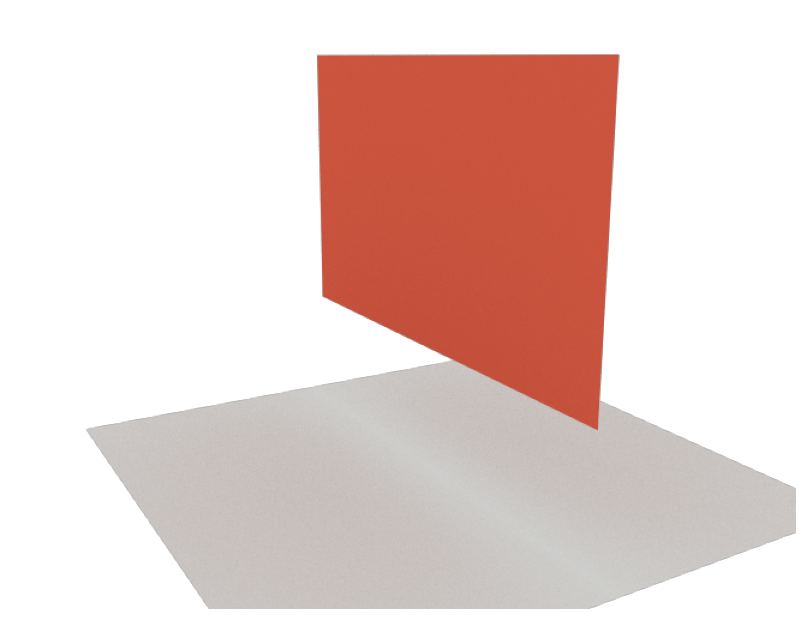
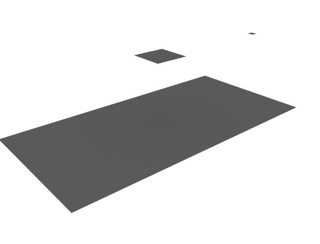
floor_wall

sionna.rt.scene.floor_wall

Example scene containing a ground plane and a vertical wall

(Blender file)

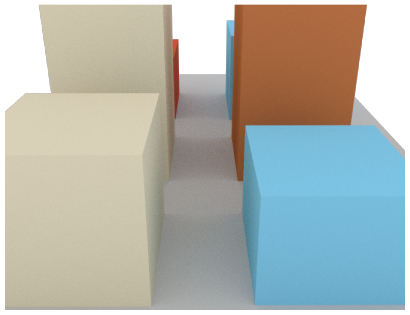
simple_street_canyon

sionna.rt.scene.simple_street_canyon

Example scene containing a few rectangular building blocks and a ground plane

(Blender file)

simple_street_canyon_with_cars

sionna.rt.scene.simple_street_canyon_with_cars

Example scene containing a few rectangular building blocks and a ground plane as well as some cars

(Blender file)

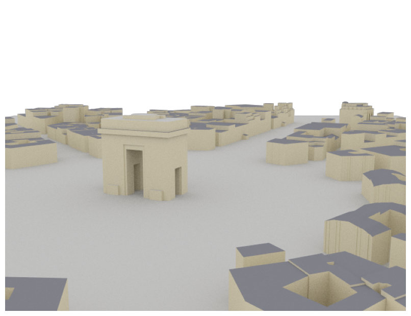
etoile

sionna.rt.scene.etoile

Example scene containing the area around the Arc de Triomphe in Paris The scene was created with data downloaded from OpenStreetMap and the help of Blender and the Blender-OSM and Mitsuba Blender add-ons. The data is licensed under the Open Data Commons Open Database License (ODbL).

(Blender file)

munich

sionna.rt.scene.munich

Example scene containing the area around the Frauenkirche in Munich The scene was created with data downloaded from OpenStreetMap and the help of Blender and the Blender-OSM and Mitsuba Blender add-ons. The data is licensed under the Open Data Commons Open Database License (ODbL).

(Blender file)

simple_wedge

sionna.rt.scene.simple_wedge

Example scene containing a wedge with a \(90^{\circ}\) opening angle

(Blender file)

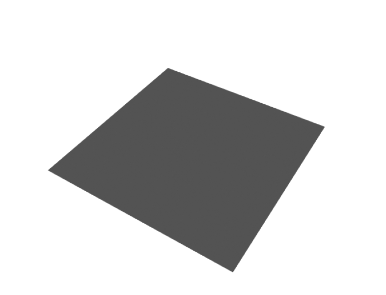
simple_reflector

sionna.rt.scene.simple_reflector

Example scene containing a metallic square

(Blender file)

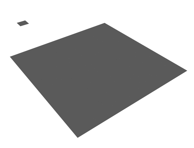
double_reflector

sionna.rt.scene.double_reflector

Example scene containing two metallic squares

(Blender file)

triple_reflector

sionna.rt.scene.triple_reflector

Example scene containing three metallic rectangles

(Blender file)

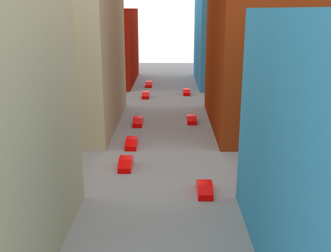
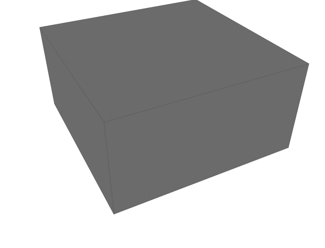
Box

sionna.rt.scene.box

Example scene containing a metallic box

(Blender file)

Paths

A propagation path \(i\) starts at a transmit antenna and ends at a receive antenna. It is described by its channel coefficient \(a_i\) and delay \(\tau_i\), as well as the angles of departure \((\theta_{\text{T},i}, \varphi_{\text{T},i})\) and arrival \((\theta_{\text{R},i}, \varphi_{\text{R},i})\). For more detail, see the Primer on Electromagnetics.

In Sionna, paths are computed with the help of the function compute_paths() which returns an instance of Paths. Paths can be visualized by providing them as arguments to the functions render(), render_to_file(), or preview().

Channel impulse responses (CIRs) can be obtained with cir() which can then be used for link-level simulations. This is for example done in the Sionna Ray Tracing Tutorial.

Paths

class sionna.rt.Paths

Stores the simulated propagation paths

Paths are generated for the loaded scene using compute_paths(). Please refer to the documentation of this function for further details. These paths can then be used to compute channel impulse responses:

paths = scene.compute_paths()
a, tau = paths.cir()

where scene is the Scene loaded using load_scene().

property a

Passband channel coefficients \(a_i\) of each path as defined in (26).

Type:

[batch_size, num_rx, num_rx_ant, num_tx, num_tx_ant, max_num_paths, num_time_steps], tf.complex

apply_doppler(sampling_frequency, num_time_steps, tx_velocities=(0.0, 0.0, 0.0), rx_velocities=(0.0, 0.0, 0.0))

Apply Doppler shifts to all paths according to the velocities of objects in the scene as well as the provided transmitter and receiver velocities.

This function replaces the last dimension of the tensor a storing the time evolution of the paths’ coefficients with a dimension of size num_time_steps.

Time evolution of the channel coefficients is simulated by computing the Doppler shift due to movements of scene objects, transmitters, and receivers. To understand this process, let us consider a single propagation path undergoing \(n\) scattering processes, such as reflection, diffuse scattering, or diffraction, as shown in the figure below.

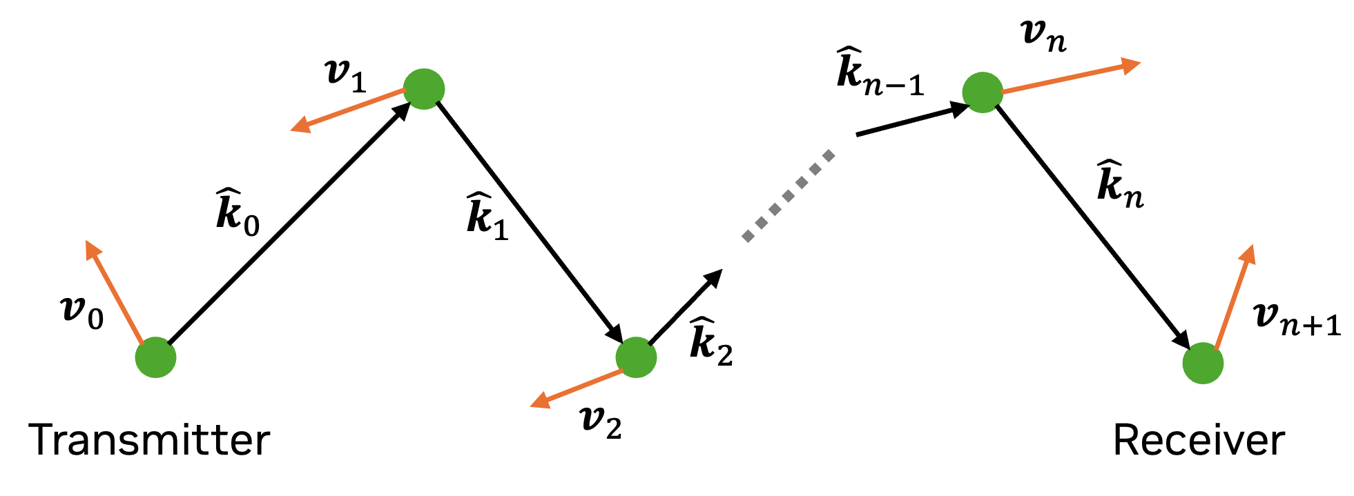
The object on which lies the \(i\text{th}\) scattering point has the velocity vector \(\hat{\mathbf{v}}_i\) and the outgoing ray direction at this point is denoted \(\hat{\mathbf{k}}_i\). The first and last point correspond to the transmitter and receiver, respectively. We therefore have

\[\begin{split}\hat{\mathbf{k}}_0 &= \hat{\mathbf{r}}(\theta_{\text{T}}, \varphi_{\text{T}})\\ \hat{\mathbf{k}}_{n} &= -\hat{\mathbf{r}}(\theta_{\text{R}}, \varphi_{\text{R}})\end{split}\]

where \((\theta_{\text{T}}, \varphi_{\text{T}})\) are the AoDs, \((\theta_{\text{R}}, \varphi_{\text{R}})\) are the AoAs, and \(\hat{\mathbf{r}}(\theta,\varphi)\) is defined in (1).

If the transmitter emits a signal with frequency \(f\), the receiver will observe the signal at frequency \(f'=f + f_\Delta\), where \(f_\Delta\) is the Doppler shift, which can be computed as [Wiffen2018]

\[f' = f \prod_{i=0}^n \frac{1 - \frac{\mathbf{v}_{i+1}^\mathsf{T}\hat{\mathbf{k}}_i}{c}}{1 - \frac{\mathbf{v}_{i}^\mathsf{T}\hat{\mathbf{k}}_i}{c}}.\]

Under the assumption that \(\lVert \mathbf{v}_i \rVert\ll c\), we can apply the Taylor expansion \((1-x)^{-1}\approx 1+x\), for \(x\ll 1\), to the previous equation to obtain

\[\begin{split}f' &\approx f \prod_{i=0}^n \left(1 - \frac{\mathbf{v}_{i+1}^\mathsf{T}\hat{\mathbf{k}}_i}{c}\right)\left(1 + \frac{\mathbf{v}_{i}^\mathsf{T}\hat{\mathbf{k}}_i}{c}\right)\\ &\approx f \left(1 + \sum_{i=0}^n \frac{\mathbf{v}_{i}^\mathsf{T}\hat{\mathbf{k}}_i -\mathbf{v}_{i+1}^\mathsf{T}\hat{\mathbf{k}}_i}{c} \right)\end{split}\]

where the second line results from ignoring terms in \(c^{-2}\). Solving for \(f_\Delta\), grouping terms with the same \(\mathbf{v}_i\) together, and using \(f=c/\lambda\), we obtain

\[f_\Delta = \frac{1}{\lambda}\left(\mathbf{v}_{0}^\mathsf{T}\hat{\mathbf{k}}_0 - \mathbf{v}_{n+1}^\mathsf{T}\hat{\mathbf{k}}_n + \sum_{i=1}^n \mathbf{v}_{i}^\mathsf{T}\left(\hat{\mathbf{k}}_i-\hat{\mathbf{k}}_{i-1} \right) \right) \qquad \text{[Hz]}.\]

Using this Doppler shift, the time-dependent path coefficient is computed as

\[a(t) = a e^{j2\pi f_\Delta t}.\]

Note that this model is only valid as long as the AoDs, AoAs, and path delays do not change significantly. This is typically the case for very short time intervals. Large-scale mobility should be simulated by moving objects within the scene and recomputing the propagation paths.

When this function is called multiple times, it overwrites the previous time step dimension.

Input:

• sampling_frequency (float) – Frequency [Hz] at which the channel impulse response is sampled

• num_time_steps (int) – Number of time steps.

• tx_velocities ([batch_size, num_tx, 3] or broadcastable, tf.float | None) – Velocity vectors \((v_\text{x}, v_\text{y}, v_\text{z})\) of all transmitters [m/s]. Defaults to [0,0,0].

• rx_velocities ([batch_size, num_rx, 3] or broadcastable, tf.float | None) – Velocity vectors \((v_\text{x}, v_\text{y}, v_\text{z})\) of all receivers [m/s]. Defaults to [0,0,0].

cir(los=True, reflection=True, diffraction=True, scattering=True, ris=True, cluster_ris_paths=True, num_paths=None)

Returns the baseband equivalent channel impulse response (28) which can be used for link simulations by other Sionna components.

The baseband equivalent channel coefficients \(a^{\text{b}}_{i}\) are computed as :

\[a^{\text{b}}_{i} = a_{i} e^{-j2 \pi f \tau_{i}}\]

where \(i\) is the index of an arbitrary path, \(a_{i}\) is the passband path coefficient (a), \(\tau_{i}\) is the path delay (tau), and \(f\) is the carrier frequency.

Note: For the paths of a given type to be returned (LoS, reflection, etc.), they must have been previously computed by compute_paths(), i.e., the corresponding flags must have been set to True.

Input:

• los (bool) – If set to False, LoS paths are not returned. Defaults to True.

• reflection (bool) – If set to False, specular paths are not returned. Defaults to True.

• diffraction (bool) – If set to False, diffracted paths are not returned. Defaults to True.

• scattering (bool) – If set to False, scattered paths are not returned. Defaults to True.

• ris (bool) – If set to False, paths involving RIS are not returned. Defaults to True.

• cluster_ris_paths (bool) – If set to True, the paths from each RIS are coherently combined into a single path, and the delays are averaged. Note that this process is performed separately for each RIS. For large RIS, clustering the paths significantly reduces the memory required to run link-level simulations. Defaults to True.

• num_paths (int or None) – All CIRs are either zero-padded or cropped to the largest num_paths paths. Defaults to None which means that no padding or cropping is done.

Output:

• a ([batch_size, num_rx, num_rx_ant, num_tx, num_tx_ant, max_num_paths, num_time_steps], tf.complex) – Path coefficients

• tau ([batch_size, num_rx, num_rx_ant, num_tx, num_tx_ant, max_num_paths] or [batch_size, num_rx, num_tx, max_num_paths], tf.float) – Path delays

property doppler

Doppler shift for each path related to movement of objects. The Doppler shifts resulting from movements of the transmitters or receivers will be computed from the inputs to the function apply_doppler().

Type:

[batch_size, num_rx, num_rx_ant, num_tx, num_tx_ant, max_num_paths] or [batch_size, num_rx, num_tx, max_num_paths], tf.float

export(filename)

Saves the paths as an OBJ file for visualisation, e.g., in Blender

Input:

filename (str) – Path and name of the file

from_dict(data_dict)

Set the paths from a dictionary which values are tensors

The format of the dictionary is expected to be the same as the one returned by to_dict().

Input:

data_dict (dict)

property mask

Set to False for non-existent paths. When there are multiple transmitters or receivers, path counts may vary between links. This is used to identify non-existent paths. For such paths, the channel coefficient is set to 0 and the delay to -1.

Type:

[batch_size, num_rx, num_rx_ant, num_tx, num_tx_ant, max_num_paths] or [batch_size, num_rx, num_tx, max_num_paths], tf.bool

property normalize_delays

Set to True to normalize path delays such that the first path between any pair of antennas of a transmitter and receiver arrives at tau = 0. Defaults to True.

Type:

bool

property phi_r

Azimuth angles of arrival [rad]

Type:

[batch_size, num_rx, num_rx_ant, num_tx, num_tx_ant, max_num_paths] or [batch_size, num_rx, num_tx, max_num_paths], tf.float

property phi_t

Azimuth angles of departure [rad]

Type:

[batch_size, num_rx, num_rx_ant, num_tx, num_tx_ant, max_num_paths] or [batch_size, num_rx, num_tx, max_num_paths], tf.float

property reverse_direction

If set to True, swaps receivers and transmitters

Type:

bool

property tau

Propagation delay \(\tau_i\) [s] of each path as defined in (26).

Type:

[batch_size, num_rx, num_rx_ant, num_tx, num_tx_ant, max_num_paths] or [batch_size, num_rx, num_tx, max_num_paths], tf.float

property theta_r

Zenith angles of arrival [rad]

Type:

[batch_size, num_rx, num_rx_ant, num_tx, num_tx_ant, max_num_paths] or [batch_size, num_rx, num_tx, max_num_paths], tf.float

property theta_t

Zenith angles of departure [rad]

Type:

[batch_size, num_rx, num_rx_ant, num_tx, num_tx_ant, max_num_paths] or [batch_size, num_rx, num_tx, max_num_paths], tf.float

to_dict()

Returns the properties of the paths as a dictionary which values are tensors

Output:

dict

property types

Type of the paths:

• 0 : LoS

• 1 : Reflected

• 2 : Diffracted

• 3 : Scattered

• 4 : RIS

Type:

[batch_size, max_num_paths], tf.int

Coverage Maps

A coverage map describes a metric, such as path gain, received signal strength (RSS), or signal-to-interference-plus-noise ratio (SINR) for a specific transmitter at every point on a plane. In other words, for a given transmitter, it associates every point on a surface with the channel gain, RSS, or SINR, that a receiver with a specific orientation would observe at this point. A coverage map is not uniquely defined as it depends on the transmit and receive arrays and their respective antenna patterns, the transmitter and receiver orientations, as well as transmit precoding and receive combining vectors. Moreover, a coverage map is not continuous but discrete because the plane needs to be quantized into small rectangular bins.

In Sionna, coverage maps are computed with the help of the function sionna.rt.Scene.coverage_map() which returns an instance of CoverageMap. They can be visualized by providing them either as arguments to the functions render(), render_to_file(), and preview(), or by using the class method show().

A very useful feature is sample_positions() which allows sampling of random positions within the scene that have sufficient path gain, RSS, or SINR from a specific transmitter. This feature is used in the Sionna Ray Tracing Tutorial to generate a dataset of channel impulse responses for link-level simulations.

CoverageMap

class sionna.rt.CoverageMap

Stores the simulated coverage maps

A coverage map is generated for the loaded scene for all transmitters using coverage_map(). Please refer to the documentation of this function for further details.

Example

import sionna
from sionna.rt import load_scene, PlanarArray, Transmitter, Receiver
scene = load_scene(sionna.rt.scene.munich)

# Configure antenna array for all transmitters
scene.tx_array = PlanarArray(num_rows=8,
                          num_cols=2,
                          vertical_spacing=0.7,
                          horizontal_spacing=0.5,
                          pattern="tr38901",
                          polarization="VH")

# Configure antenna array for all receivers
scene.rx_array = PlanarArray(num_rows=1,
                          num_cols=1,
                          vertical_spacing=0.5,
                          horizontal_spacing=0.5,
                          pattern="dipole",
                          polarization="cross")
# Add a transmitters
tx = Transmitter(name="tx",
              position=[8.5,21,30],
              orientation=[0,0,0])
scene.add(tx)
tx.look_at([40,80,1.5])

# Compute coverage map
cm = scene.coverage_map(max_depth=8)

# Show coverage map
cm.show();

cdf(metric='path_gain', tx=None)

Computes and visualizes the CDF of a metric of the coverage map

Input:

• metric (str, one of [“path_gain”, “rss”, “sinr”]) – Metric to be shown. Defaults to “path_gain”.

• tx (int | str | None) – Index or name of the transmitter for which to show the coverage map. If None, the maximum value over all transmitters for each cell is shown. Defaults to None.

Output:

• Figure – Figure showing the CDF

• x (tf.float, [num_cells_x * num_cells_y]) – Data points for the chosen metric

• cdf (tf.float, [num_cells_x * num_cells_y]) – Cummulative probabilities for the data points

property cell_centers

Positions of the centers of the cells in the global coordinate system

Type:

[num_cells_y, num_cells_x, 3], tf.float

property cell_size

Resolution of the coverage map, i.e., width (in the local X direction) and height (in the local Y direction) in of the cells of the coverage map

Type:

[2], tf.float

cell_to_tx(metric)

Computes cell-to-transmitter association. Each cell is associated with the transmitter providing the highest metric, such as path gain, received signal strength (RSS), or SINR.

Input:

metric (str, one of [“path_gain”, “rss”, “sinr”]) – Metric to be used

Output:

cell_to_tx ([num_cells_y, num_cells_x], tf.int64) – Cell-to-transmitter association

property center

Center of the coverage map in the global coordinate system

Type:

[3], tf.float

property num_cells_x

Number of cells along the local X-axis

Type:

int

property num_cells_y

Number of cells along the local Y-axis

Type:

int

property num_tx

Number of transmitters

Type:

int

property orientation

Orientation of the coverage map \((\alpha, \beta, \gamma)\) specified through three angles corresponding to a 3D rotation as defined in (3). An orientation of \((0,0,0)\) corresponds to a coverage map that is parallel to the XY plane.

Type:

[3], tf.float

property path_gain

Path gains across the coverage map from all transmitters

Type:

[num_tx, num_cells_y, num_cells_x], tf.float

property ris_pos

(column, row) cell index position of each RIS

Type:

[num_ris, 2], int

property rss

Received signal strength (RSS) across the coverage map from all transmitters

Type:

[num_tx, num_cells_y, num_cells_x], tf.float

property rx_pos

(column, row) cell index position of each receiver

Type:

[num_rx, 2], int

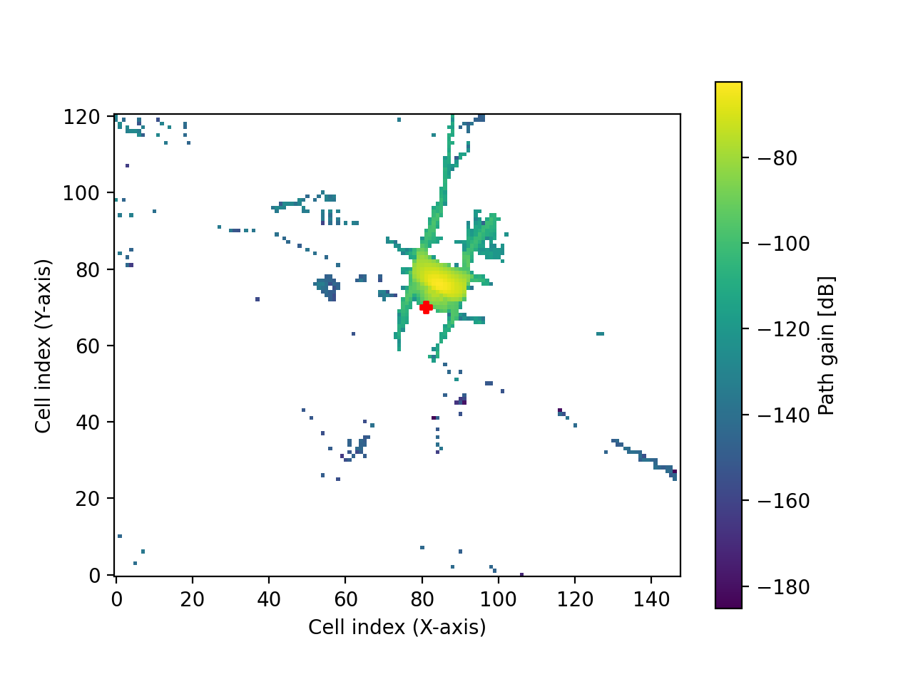
sample_positions(num_pos, metric='path_gain', min_val_db=None, max_val_db=None, min_dist=None, max_dist=None, tx_association=True, center_pos=False)

Sample random user positions in a scene based on a coverage map

For a given coverage map, num_pos random positions are sampled around each transmitter, such that the selected metric, e.g., SINR, is larger than min_val_db and/or smaller than max_val_db. Similarly, min_dist and max_dist define the minimum and maximum distance of the random positions to the transmitter under consideration. By activating the flag tx_association, only positions are sampled for which the selected metric is the highest across all transmitters. This is useful if one wants to ensure, e.g., that the sampled positions for each transmitter provide the highest SINR or RSS.

Note that due to the quantization of the coverage map into cells it is not guaranteed that all above parameters are exactly fulfilled for a returned position. This stems from the fact that every individual cell of the coverage map describes the expected average behavior of the surface within this cell. For instance, it may happen that half of the selected cell is shadowed and, thus, no path to the transmitter exists but the average path gain is still larger than the given threshold. Please enable the flag center_pos to sample only positions from the cell centers.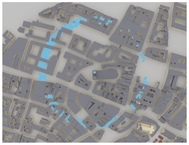

The above figure shows an example for random positions between 220m and 250m from the transmitter and a maximum path gain of -100 dB. Keep in mind that the transmitter can have a different height than the coverage map which also contributes to this distance. For example if the transmitter is located 20m above the surface of the coverage map and a min_dist of 20m is selected, also positions directly below the transmitter are sampled.

Input:

• num_pos (int) – Number of returned random positions for ech transmitter

• metric (str, one of [“path_gain”, “rss”, “sinr”]) – Metric to be considered for sampling positions. Defaults to “path_gain”.

• min_val_db (float | None) – Minimum value for the selected metric ([dB] for path gain and SINR; [dBm] for RSS). Positions are only sampled from cells where the selected metric is larger than or equal to this value. Ignored if None. Defaults to None.

• max_val_db (float | None) – Maximum value for the selected metric ([dB] for path gain and SINR; [dBm] for RSS). Positions are only sampled from cells where the selected metric is smaller than or equal to this value. Ignored if None. Defaults to None.

• min_dist (float | None) – Minimum distance [m] from transmitter for all random positions. Ignored if None. Defaults to None.

• max_dist (float | None) – Maximum distance [m] from transmitter for all random positions. Ignored if None. Defaults to None.

• tx_association (bool) – If True, only positions associated with a transmitter are chosen, i.e., positions where the chosen metric is the highest among all all transmitters. Else, a user located in a sampled position for a specific transmitter may perceive a higher metric from another TX. Defaults to True.

• center_pos (bool) – If True, all returned positions are sampled from the cell center (i.e., the grid of the coverage map). Otherwise, the positions are randomly drawn from the surface of the cell. Defaults to False.

Output:

• [num_tx, num_pos, 3], tf.float – Random positions \((x,y,z)\) [m] that are in cells fulfilling the configured constraints

• [num_tx, num_pos, 2], tf.float – Cell indices corresponding to the random positions

show(metric='path_gain', tx=None, vmin=None, vmax=None, show_tx=True, show_rx=False, show_ris=False)

Visualizes a coverage map

The position of the transmitter is indicated by a red “+” marker. The positions of the receivers are indicated by blue “x” markers. The positions of the RIS are indicated by black “*” markers.

Input:

• metric (str, one of [“path_gain”, “rss”, “sinr”]) – Metric to be shown. Defaults to “path_gain”.

• tx (int | str | None) – Index or name of the transmitter for which to show the coverage map. If None, the maximum value over all transmitters for each cell is shown. Defaults to None.

• vmin,vmax (float | None) – Define the range of values [dB] that the colormap covers. If set to None, the complete range is shown. Defaults to None.

• show_tx (bool) – If set to True, then the position of the transmitters are shown. Defaults to True.

• show_rx (bool) – If set to True, then the position of the receivers are shown. Defaults to False.

• show_ris (bool) – If set to True, then the position of the RIS are shown. Defaults to False.

Output:

Figure – Figure showing the coverage map

show_association(metric='path_gain', show_tx=True, show_rx=False, show_ris=False)

Visualizes cell-to-tx association for a given metric

The position of the transmitter is indicated by a red “+” marker. The positions of the receivers are indicated by blue “x” markers. The positions of the RIS are indicated by black “*” markers.

Input:

• metric (str, one of [“path_gain”, “rss”, “sinr”]) – Metric based on which the cell-to-tx association is computed. Defaults to “path_gain”.

• show_tx (bool) – If set to True, then the position of the transmitters are shown. Defaults to True.

• show_rx (bool) – If set to True, then the position of the receivers are shown. Defaults to False.

• show_ris (bool) – If set to True, then the position of the RIS are shown. Defaults to False.

Output:

Figure – Figure showing the cell-to-transmitter association

property sinr

SINR across the coverage map from all transmitters

Type:

[num_tx, num_cells_y, num_cells_x], tf.float

property size

Size of the coverage map

Type:

[2], tf.float

property tx_pos

(column, row) cell index position of each transmitter

Type:

[num_tx, 2], int

Cameras

A Camera defines a position and view direction for rendering the scene.

The cameras property of the Scene list all the cameras currently available for rendering. Cameras can be either defined through the scene file or instantiated using the API. The following code snippet shows how to load a scene and list the available cameras:

scene = load_scene(sionna.rt.scene.munich)
print(scene.cameras)
scene.render("scene-cam-0") # Use the first camera of the scene for rendering

A new camera can be instantiated as follows:

cam = Camera("mycam", position=[200., 0.0, 50.])
scene.add(cam)
cam.look_at([0.0,0.0,0.0])
scene.render(cam) # Render using the Camera instance
scene.render("mycam") # or using the name of the camera

Camera

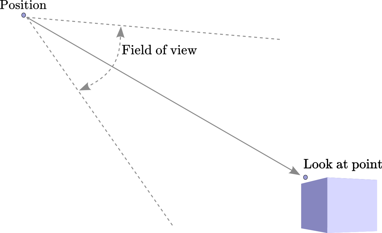
class sionna.rt.Camera(name, position, orientation=[0., 0., 0.], look_at=None)

A camera defines a position and view direction for rendering the scene.

In its local coordinate system, a camera looks toward the positive X-axis with the positive Z-axis being the upward direction.

Input:

• name (str) – Name. Cannot be “preview”, as it is reserved for the viewpoint of the interactive viewer.

• position ([3], float) – Position \((x,y,z)\) [m] as three-dimensional vector

• orientation ([3], float) – Orientation \((\alpha, \beta, \gamma)\) specified through three angles corresponding to a 3D rotation as defined in (3). This parameter is ignored if look_at is not None. Defaults to [0,0,0].

• look_at ([3], float | Transmitter | Receiver | RIS | Camera | None) – A position or the instance of a Transmitter, Receiver, RIS, or Camera to look at. If set to None, then orientation is used to orientate the device.

look_at(target)

Sets the orientation so that the camera looks at a position, radio device, or another camera.

Given a point \(\mathbf{x}\in\mathbb{R}^3\) with spherical angles \(\theta\) and \(\varphi\), the orientation of the camera will be set equal to \((\varphi, \frac{\pi}{2}-\theta, 0.0)\).

Input:

target ([3], float | Transmitter | Receiver | Camera | str) – A position or the name or instance of a Transmitter, Receiver, or Camera in the scene to look at.

property orientation

Get/set the orientation \((\alpha, \beta, \gamma)\) specified through three angles corresponding to a 3D rotation as defined in (3).

Type:

[3], float

property position

Get/set the position \((x,y,z)\) as three-dimensional vector

Type:

[3], float

Scene Objects

A scene is made of scene objects. Examples include cars, trees, buildings, furniture, etc. A scene object is characterized by its geometry and material (RadioMaterial) and implemented as an instance of the SceneObject class.

Scene objects are uniquely identified by their name. To access a scene object, the get() method of Scene may be used. For example, the following code snippet shows how to load a scene and list its scene objects:

scene = load_scene(sionna.rt.scene.munich)
print(scene.objects)

To select an object, e.g., named “Schrannenhalle-itu_metal”, you can run:

my_object = scene.get("Schrannenhalle-itu_metal")

You can then set the RadioMaterial of my_object as follows:

my_object.radio_material = "itu_wood"

Most scene objects names have postfixes of the form “-material_name”. These are used during loading of a scene to assign a RadioMaterial to each of them. This tutorial video explains how you can assign radio materials to objects when you create your own scenes.

SceneObject

class sionna.rt.SceneObject

Every object in the scene is implemented by an instance of this class

look_at(target)

Sets the orientation so that the x-axis points toward an Object.

Input:

target ([3], float | sionna.rt.Object | str) – A position or the name or instance of an sionna.rt.Object in the scene to point toward to

property name

Name

Type:

str (read-only)

property orientation

Get/set the orientation \((\alpha, \beta, \gamma)\) [rad] specified through three angles corresponding to a 3D rotation as defined in (3).

Type:

[3], tf.float

property position

Get/set the position vector [m] of the center of the object. The center is defined as the object’s axis-aligned bounding box (AABB).

Type:

[3], tf.float

property radio_material

Get/set the radio material of the object. Setting can be done by using either an instance of RadioMaterial or the material name (str). If the radio material is not part of the scene, it will be added. This can raise an error if a different radio material with the same name was already added to the scene.

Type:

RadioMaterial

property velocity

Get/set the velocity vector [m/s]

Type:

[3], tf.float

Radio Materials

A RadioMaterial contains everything that is needed to enable the simulation of the interaction of a radio wave with an object made of a particular material. More precisely, it consists of the real-valued relative permittivity \(\varepsilon_r\), the conductivity \(\sigma\), and the relative permeability \(\mu_r\). For more details, see (7), (8), (9). These quantities can possibly depend on the frequency of the incident radio wave. Note that Sionna currently only allows non-magnetic materials with \(\mu_r=1\).

Additionally, a RadioMaterial can have an effective roughness (ER) associated with it, leading to diffuse reflections (see, e.g., [Degli-Esposti11]). The ER model requires a scattering coefficient \(S\in[0,1]\) (37), a cross-polarization discrimination coefficient \(K_x\) (39), as well as a scattering pattern \(f_\text{s}(\hat{\mathbf{k}}_\text{i}, \hat{\mathbf{k}}_\text{s})\) (40)–(42), such as the LambertianPattern or DirectivePattern. The meaning of these parameters is explained in Scattering.

Similarly to scene objects (SceneObject), all radio materials are uniquely identified by their name. For example, specifying that a scene object named “wall” is made of the material named “itu-brick” is done as follows:

obj = scene.get("wall") # obj is a SceneObject
obj.radio_material = "itu_brick" # "wall" is made of "itu_brick"

Sionna provides the ITU models of several materials whose properties are automatically updated according to the configured frequency. It is also possible to define custom radio materials.

Radio materials provided with Sionna

Sionna provides the models of all of the materials defined in the ITU-R P.2040-2 recommendation [ITUR_P2040_2]. These models are based on curve fitting to measurement results and assume non-ionized and non-magnetic materials (\(\mu_r = 1\)). Frequency dependence is modeled by

\[\begin{split}\begin{align} \varepsilon_r &= a f_{\text{GHz}}^b\\ \sigma &= c f_{\text{GHz}}^d \end{align}\end{split}\]

where \(f_{\text{GHz}}\) is the frequency in GHz, and the constants \(a\), \(b\), \(c\), and \(d\) characterize the material. The table below provides their values which are used in Sionna (from [ITUR_P2040_2]). Note that the relative permittivity \(\varepsilon_r\) and conductivity \(\sigma\) of all materials are updated automatically when the frequency is set through the scene’s property frequency. Moreover, by default, the scattering coefficient, \(S\), of these materials is set to 0, leading to no diffuse reflection.

Material name	Real part of relative permittivity		Conductivity [S/m]		Frequency range (GHz)
	a	b	c	d
vacuum	1	0	0	0	0.001 – 100
itu_concrete	5.24	0	0.0462	0.7822	1 – 100
itu_brick	3.91	0	0.0238	0.16	1 – 40
itu_plasterboard	2.73	0	0.0085	0.9395	1 – 100
itu_wood	1.99	0	0.0047	1.0718	0.001 – 100
itu_glass	6.31	0	0.0036	1.3394	0.1 – 100
	5.79	0	0.0004	1.658	220 – 450
itu_ceiling_board	1.48	0	0.0011	1.0750	1 – 100
	1.52	0	0.0029	1.029	220 – 450
itu_chipboard	2.58	0	0.0217	0.7800	1 – 100
itu_plywood	2.71	0	0.33	0	1 – 40
itu_marble	7.074	0	0.0055	0.9262	1 – 60
itu_floorboard	3.66	0	0.0044	1.3515	50 – 100
itu_metal	1	0	\(10^7\)	0	1 – 100
itu_very_dry_ground	3	0	0.00015	2.52	1 – 10
itu_medium_dry_ground	15	-0.1	0.035	1.63	1 – 10
itu_wet_ground	30	-0.4	0.15	1.30	1 – 10

Defining custom radio materials

Custom radio materials can be implemented using the RadioMaterial class by specifying a relative permittivity \(\varepsilon_r\) and conductivity \(\sigma\), as well as optional parameters related to diffuse scattering, such as the scattering coefficient \(S\), cross-polarization discrimination coefficient \(K_x\), and scattering pattern \(f_\text{s}(\hat{\mathbf{k}}_\text{i}, \hat{\mathbf{k}}_\text{s})\). Note that only non-magnetic materials with \(\mu_r=1\) are currently allowed. The following code snippet shows how to create a custom radio material.

load_scene() # Load empty scene
custom_material = RadioMaterial("my_material",
                                relative_permittivity=2.0,
                                conductivity=5.0,
                                scattering_coefficient=0.3,
                                xpd_coefficient=0.1,
                                scattering_pattern=LambertianPattern())

It is also possible to define the properties of a material through a callback function that computes the material properties \((\varepsilon_r, \sigma)\) from the frequency:

def my_material_callback(f_hz):
   relative_permittivity = compute_relative_permittivity(f_hz)
   conductivity = compute_conductivity(f_hz)
   return (relative_permittivity, conductivity)

custom_material = RadioMaterial("my_material",
                                frequency_update_callback=my_material_callback)
scene.add(custom_material)

Once defined, the custom material can be assigned to a SceneObject using its name:

obj = scene.get("my_object") # obj is a SceneObject
obj.radio_material = "my_material" # "my_object" is made of "my_material"

or the material instance:

obj = scene.get("my_object") # obj is a SceneObject
obj.radio_material = custom_material # "my_object" is made of "my_material"

The material parameters can be assigned to TensorFlow variables or tensors, such as the output of a Keras layer defining a neural network. This allows one to make materials trainable:

mat = RadioMaterial("my_mat",
                    relative_permittivity= tf.Variable(2.1, dtype=tf.float32))
mat.conductivity = tf.Variable(0.0, dtype=tf.float32)

RadioMaterial

class sionna.rt.RadioMaterial(name, relative_permittivity=1.0, conductivity=0.0, scattering_coefficient=0.0, xpd_coefficient=0.0, scattering_pattern=None, frequency_update_callback=None, dtype=tf.complex64)

Class implementing a radio material

A radio material is defined by its relative permittivity \(\varepsilon_r\) and conductivity \(\sigma\) (see (9)), as well as optional parameters related to diffuse scattering, such as the scattering coefficient \(S\), cross-polarization discrimination coefficient \(K_x\), and scattering pattern \(f_\text{s}(\hat{\mathbf{k}}_\text{i}, \hat{\mathbf{k}}_\text{s})\).

We assume non-ionized and non-magnetic materials, and therefore the permeability \(\mu\) of the material is assumed to be equal to the permeability of vacuum i.e., \(\mu_r=1.0\).

For frequency-dependent materials, it is possible to specify a callback function frequency_update_callback that computes the material properties \((\varepsilon_r, \sigma)\) from the frequency. If a callback function is specified, the material properties cannot be set and the values specified at instantiation are ignored. The callback should return -1 for both the relative permittivity and the conductivity if these are not defined for the given carrier frequency.

The material properties can be assigned to a TensorFlow variable or tensor. In the latter case, the tensor could be the output of a callable, such as a Keras layer implementing a neural network. In the former case, it could be set to a trainable variable:

mat = RadioMaterial("my_mat")
mat.conductivity = tf.Variable(0.0, dtype=tf.float32)

Parameters:

• name (str) – Unique name of the material

• relative_permittivity (float | None) – Relative permittivity of the material. Must be larger or equal to 1. Defaults to 1. Ignored if frequency_update_callback is provided.

• conductivity (float | None) – Conductivity of the material [S/m]. Must be non-negative. Defaults to 0. Ignored if frequency_update_callback is provided.

• scattering_coefficient (float) – Scattering coefficient \(S\in[0,1]\) as defined in (37). Defaults to 0.

• xpd_coefficient (float) – Cross-polarization discrimination coefficient \(K_x\in[0,1]\) as defined in (39). Only relevant if scattering_coefficient>0. Defaults to 0.

• scattering_pattern (ScatteringPattern) – ScatteringPattern to be applied. Only relevant if scattering_coefficient>0. Defaults to None, which implies a LambertianPattern.

• frequency_update_callback (callable | None) –

  An optional callable object used to obtain the material parameters from the scene’s frequency. This callable must take as input the frequency [Hz] and must return the material properties as a tuple:

  (relative_permittivity, conductivity).

  If set to None, the material properties are constant and equal to relative_permittivity and conductivity. Defaults to None.

• dtype (tf.complex64 or tf.complex128) – Datatype. Defaults to tf.complex64.

property complex_relative_permittivity

Complex relative permittivity \(\eta\) (9)

Type:

tf.complex (read-only)

property conductivity

Get/set the conductivity \(\sigma\) [S/m] (9)

Type:

tf.float

property frequency_update_callback

Get/set frequency update callback function

Type:

callable

property is_used

Indicator if the material is used by at least one object of the scene

Type:

bool

property name

Name of the radio material

Type:

str (read-only)

property relative_permeability

Relative permeability \(\mu_r\) (8). Defaults to 1.

Type:

tf.float (read-only)

property relative_permittivity

Get/set the relative permittivity \(\varepsilon_r\) (9)

Type:

tf.float

property scattering_coefficient

Get/set the scattering coefficient \(S\in[0,1]\) (37).

Type:

tf.float

property scattering_pattern

Get/set the ScatteringPattern.

Type:

ScatteringPattern

property use_counter

Number of scene objects using this material

Type:

int

property using_objects

Identifiers of the objects using this material

Type:

[num_using_objects], tf.int

property well_defined

Get if the material is well-defined

Type:

bool

property xpd_coefficient

Get/set the cross-polarization discrimination coefficient \(K_x\in[0,1]\) (39).

Type:

tf.float

ScatteringPattern

class sionna.rt.LambertianPattern(dtype=tf.complex64)

Lambertian scattering model from [Degli-Esposti07] as given in (40)

Parameters:

dtype (tf.complex64 or tf.complex128) – Datatype used for all computations. Defaults to tf.complex64.

Input:

• k_i ([batch_size, 3], dtype.real_dtype) – Incoming directions

• k_s ([batch_size,3], dtype.real_dtype) – Outgoing directions

Output:

pattern ([batch_size], dtype.real_dtype) – Scattering pattern

Example

>>> LambertianPattern().visualize()

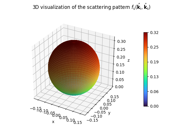
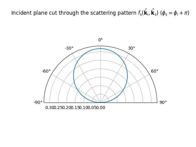
visualize(k_i=(0.7071, 0.0, -0.7071), show_directions=False)

Visualizes the scattering pattern

It is assumed that the surface normal points toward the positive z-axis.

Input:

• k_i ([3], array_like) – Incoming direction

• show_directions (bool) – If True, the incoming and specular reflection directions are shown. Defaults to False.

Output:

• matplotlib.pyplot.Figure – 3D visualization of the scattering pattern

• matplotlib.pyplot.Figure – Visualization of the incident plane cut through the scattering pattern

class sionna.rt.DirectivePattern(alpha_r, dtype=tf.complex64)

Directive scattering model from [Degli-Esposti07] as given in (41)

Parameters:

• alpha_r (int, [1,2,...]) – Parameter related to the width of the scattering lobe in the direction of the specular reflection.

• dtype (tf.complex64 or tf.complex128) – Datatype used for all computations. Defaults to tf.complex64.

Input:

• k_i ([batch_size, 3], dtype.real_dtype) – Incoming directions

• k_s ([batch_size,3], dtype.real_dtype) – Outgoing directions

Output:

pattern ([batch_size], dtype.real_dtype) – Scattering pattern

Example

>>> DirectivePattern(alpha_r=10).visualize()

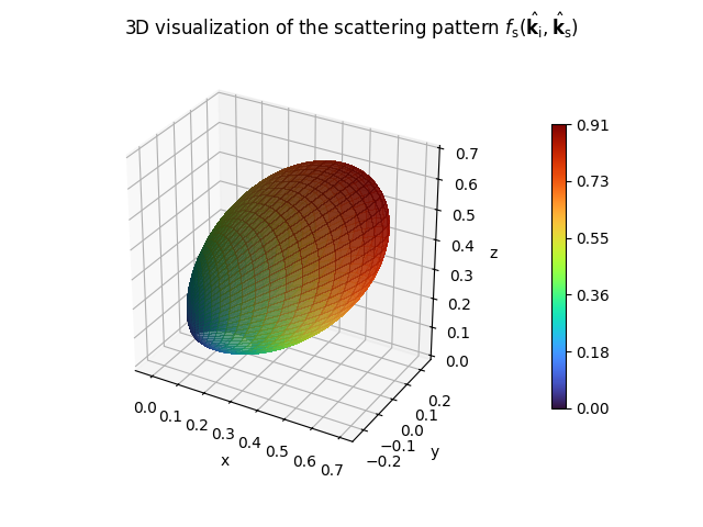
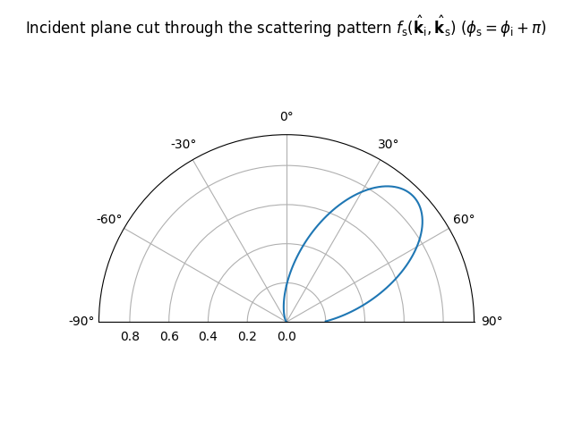
property alpha_r

Get/set alpha_r

Type:

bool

visualize(k_i=(0.7071, 0.0, -0.7071), show_directions=False)

Visualizes the scattering pattern

It is assumed that the surface normal points toward the positive z-axis.

Input:

• k_i ([3], array_like) – Incoming direction

• show_directions (bool) – If True, the incoming and specular reflection directions are shown. Defaults to False.

Output:

• matplotlib.pyplot.Figure – 3D visualization of the scattering pattern

• matplotlib.pyplot.Figure – Visualization of the incident plane cut through the scattering pattern

class sionna.rt.BackscatteringPattern(alpha_r, alpha_i, lambda_, dtype=tf.complex64)

Backscattering model from [Degli-Esposti07] as given in (42)

The parameter lambda_ can be assigned to a TensorFlow variable or tensor. In the latter case, the tensor can be the output of a callable, such as a Keras layer implementing a neural network. In the former case, it can be set to a trainable variable:

sp = BackscatteringPattern(alpha_r=3,
                           alpha_i=5,
                           lambda_=tf.Variable(0.3, dtype=tf.float32))

Parameters:

• alpha_r (int, [1,2,...]) – Parameter related to the width of the scattering lobe in the direction of the specular reflection.

• alpha_i (int, [1,2,...]) – Parameter related to the width of the scattering lobe in the incoming direction.

• lambda (float, [0,1]) – Parameter determining the percentage of the diffusely reflected energy in the lobe around the specular reflection.

• dtype (tf.complex64 or tf.complex128) – Datatype used for all computations. Defaults to tf.complex64.

Input:

• k_i ([batch_size, 3], dtype.real_dtype) – Incoming directions

• k_s ([batch_size,3], dtype.real_dtype) – Outgoing directions

Output:

pattern ([batch_size], dtype.real_dtype) – Scattering pattern

Example

>>> BackscatteringPattern(alpha_r=20, alpha_i=30, lambda_=0.7).visualize()

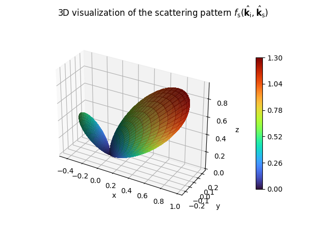
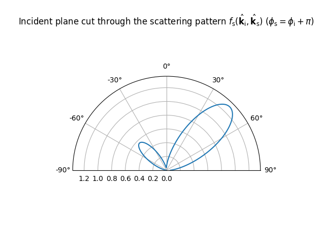
property alpha_i

Get/set alpha_i

Type:

bool

property alpha_r

Get/set alpha_r

Type:

bool

property lambda_

Get/set lambda_

Type:

bool

visualize(k_i=(0.7071, 0.0, -0.7071), show_directions=False)

Visualizes the scattering pattern

It is assumed that the surface normal points toward the positive z-axis.

Input:

• k_i ([3], array_like) – Incoming direction

• show_directions (bool) – If True, the incoming and specular reflection directions are shown. Defaults to False.

Output:

• matplotlib.pyplot.Figure – 3D visualization of the scattering pattern

• matplotlib.pyplot.Figure – Visualization of the incident plane cut through the scattering pattern

Radio Devices

A radio device refers to a Transmitter or Receiver equipped with an AntennaArray as specified by the Scene’s properties tx_array and rx_array, respectively. Also reconfigurable intelligent surfaces (RIS) inherit from this class.

The following code snippet shows how to instantiate a Transmitter equipped with a \(4 \times 2\) PlanarArray with cross-polarized isotropic antennas:

 scene.tx_array = PlanarArray(num_rows=4,
                              num_cols=2,
                              vertical_spacing=0.5,
                              horizontal_spacing=0.5,
                              pattern="iso",
                              polarization="cross")

 my_tx = Transmitter(name="my_tx",
                     position=(0,0,0),
                     orientation=(0,0,0))

scene.add(my_tx)

The position \((x,y,z)\) and orientation \((\alpha, \beta, \gamma)\) of a radio device can be freely configured. The latter is specified through three angles corresponding to a 3D rotation as defined in (3). Both can be assigned to TensorFlow variables or tensors. In the latter case, the tensor can be the output of a callable, such as a Keras layer implementing a neural network. In the former case, it can be set to a trainable variable.

Radio devices need to be explicitly added to the scene using the scene’s method add() and can be removed from it using remove():

scene = load_scene()
scene.add(Transmitter("tx", [10.0, 0.0, 1.5], [0.0,0.0,0.0]))
scene.remove("tx")

Transmitter

class sionna.rt.Transmitter(name, position, orientation=(0.0, 0.0, 0.0), look_at=None, power_dbm=44, color=(0.16, 0.502, 0.725), dtype=tf.complex64)

Class defining a transmitter

The position, orientation, and power_dbm properties can be assigned to a TensorFlow variable or tensor. In the latter case, the tensor can be the output of a callable, such as a Keras layer implementing a neural network. In the former case, it can be set to a trainable variable:

tx = Transmitter(name="my_tx",
                 position=tf.Variable([0, 0, 0], dtype=tf.float32),
                 orientation=tf.Variable([0, 0, 0], dtype=tf.float32),
                 power_dbm=tf.Variable(44, dtype=tf.float32))

Parameters:

• name (str) – Name

• position ([3], float) – Position \((x,y,z)\) [m] as three-dimensional vector

• power_dbm (float) – Transmit power [dBm]

• orientation ([3], float) – Orientation \((\alpha, \beta, \gamma)\) [rad] specified through three angles corresponding to a 3D rotation as defined in (3). This parameter is ignored if look_at is not None. Defaults to [0,0,0].

• look_at ([3], float | Transmitter | Receiver | RIS | Camera | None) – A position or the instance of a Transmitter, Receiver, RIS, or Camera to look at. If set to None, then orientation is used to orientate the device.

• color ([3], float) – Defines the RGB (red, green, blue) color parameter for the device as displayed in the previewer and renderer. Each RGB component must have a value within the range \(\in [0,1]\). Defaults to [0.160, 0.502, 0.725].

• dtype (tf.complex) – Datatype to be used in internal calculations. Defaults to tf.complex64.

property color

Get/set the the RGB (red, green, blue) color for the device as displayed in the previewer and renderer. Each RGB component must have a value within the range \(\in [0,1]\).

Type:

[3], float

look_at(target)

Sets the orientation so that the x-axis points toward a position, radio device, RIS, or camera.

Given a point \(\mathbf{x}\in\mathbb{R}^3\) with spherical angles \(\theta\) and \(\varphi\), the orientation of the radio device will be set equal to \((\varphi, \frac{\pi}{2}-\theta, 0.0)\).

Input:

target ([3], float | Transmitter | Receiver | RIS | Camera | str) – A position or the name or instance of a Transmitter, Receiver, RIS, or Camera in the scene to look at.

property name

Name

Type:

str (read-only)

property orientation

Get/set the orientation

Type:

[3], tf.float

property position

Get/set the position

Type:

[3], tf.float

property power

Get the transmit power [W]

Type:

tf.float

property power_dbm

Get/set transmit power [dBm]

Type:

tf.float

Receiver

class sionna.rt.Receiver(name, position, orientation=(0.0, 0.0, 0.0), look_at=None, color=(0.153, 0.682, 0.375), dtype=tf.complex64)

Class defining a receiver

The position and orientation properties can be assigned to a TensorFlow variable or tensor. In the latter case, the tensor can be the output of a callable, such as a Keras layer implementing a neural network. In the former case, it can be set to a trainable variable:

rx = Transmitter(name="my_rx",
                 position=tf.Variable([0, 0, 0], dtype=tf.float32),
                 orientation=tf.Variable([0, 0, 0], dtype=tf.float32))

Parameters:

• name (str) – Name

• position ([3], float) – Position \((x,y,z)\) as three-dimensional vector

• orientation ([3], float) – Orientation \((\alpha, \beta, \gamma)\) [rad] specified through three angles corresponding to a 3D rotation as defined in (3). This parameter is ignored if look_at is not None. Defaults to [0,0,0].

• look_at ([3], float | Transmitter | Receiver | RIS | Camera | None) – A position or the instance of a Transmitter, Receiver, RIS, or Camera to look at. If set to None, then orientation is used to orientate the device.

• color ([3], float) – Defines the RGB (red, green, blue) color parameter for the device as displayed in the previewer and renderer. Each RGB component must have a value within the range \(\in [0,1]\). Defaults to [0.153, 0.682, 0.375].

• dtype (tf.complex) – Datatype to be used in internal calculations. Defaults to tf.complex64.

property color

Get/set the the RGB (red, green, blue) color for the device as displayed in the previewer and renderer. Each RGB component must have a value within the range \(\in [0,1]\).

Type:

[3], float

look_at(target)

Sets the orientation so that the x-axis points toward a position, radio device, RIS, or camera.

Given a point \(\mathbf{x}\in\mathbb{R}^3\) with spherical angles \(\theta\) and \(\varphi\), the orientation of the radio device will be set equal to \((\varphi, \frac{\pi}{2}-\theta, 0.0)\).

Input:

target ([3], float | Transmitter | Receiver | RIS | Camera | str) – A position or the name or instance of a Transmitter, Receiver, RIS, or Camera in the scene to look at.

property name

Name

Type:

str (read-only)

property orientation

Get/set the orientation

Type:

[3], tf.float

property position

Get/set the position

Type:

[3], tf.float

Antenna Arrays

Transmitters (Transmitter) and receivers (Receiver) are equipped with an AntennaArray that is composed of one or more antennas. All transmitters and all receivers share the same AntennaArray which can be set through the scene properties tx_array and rx_array, respectively.

AntennaArray

class sionna.rt.AntennaArray(antenna, positions, dtype=tf.complex64)

Class implementing an antenna array

An antenna array is composed of identical antennas that are placed at different positions. The positions parameter can be assigned to a TensorFlow variable or tensor.

array = AntennaArray(antenna=Antenna("tr38901", "V"),
                     positions=tf.Variable([[0,0,0], [0, 1, 1]]))

Parameters:

• antenna (Antenna) – Antenna instance

• positions ([array_size, 3], array_like) – Array of relative positions \((x,y,z)\) [m] of each antenna (dual-polarized antennas are counted as a single antenna and share the same position). The absolute position of the antennas is obtained by adding the position of the Transmitter or Receiver using it.

• dtype (tf.complex64 or tf.complex128) – Data type used for all computations. Defaults to tf.complex64.

property antenna

Get/set the antenna

Type:

Antenna

property array_size

Number of antennas in the array. Dual-polarized antennas are counted as a single antenna.

Type:

int (read-only)

property num_ant

Number of linearly polarized antennas in the array. Dual-polarized antennas are counted as two linearly polarized antennas.

Type:

int (read-only)

property positions

Get/set array of relative positions \((x,y,z)\) [m] of each antenna (dual-polarized antennas are counted as a single antenna and share the same position).

Type:

[array_size, 3], tf.float

rotated_positions(orientation)

Get the antenna positions rotated according to orientation

Input:

orientation ([3], tf.float) – Orientation \((\alpha, \beta, \gamma)\) [rad] specified through three angles corresponding to a 3D rotation as defined in (3).

Output:

[array_size, 3] – Rotated positions

PlanarArray

class sionna.rt.PlanarArray(num_rows, num_cols, vertical_spacing, horizontal_spacing, pattern, polarization=None, polarization_model=2, dtype=tf.complex64)

Class implementing a planar antenna array

The antennas are regularly spaced, located in the y-z plane, and numbered column-first from the top-left to bottom-right corner.

Parameters:

• num_rows (int) – Number of rows

• num_cols (int) – Number of columns

• vertical_spacing (float) – Vertical antenna spacing [multiples of wavelength].

• horizontal_spacing (float) – Horizontal antenna spacing [multiples of wavelength].

• pattern (str, callable, or length-2 sequence of callables) – Antenna pattern. Either one of [“iso”, “dipole”, “hw_dipole”, “tr38901”], or a callable, or a length-2 sequence of callables defining antenna patterns. In the latter case, the antennas are dual polarized and each callable defines the antenna pattern in one of the two orthogonal polarization directions. An antenna pattern is a callable that takes as inputs vectors of zenith and azimuth angles of the same length and returns for each pair the corresponding zenith and azimuth patterns. See (14) for more detail.

• polarization (str or None) – Type of polarization. For single polarization, must be “V” (vertical) or “H” (horizontal). For dual polarization, must be “VH” or “cross”. Only needed if pattern is a string.

• polarization_model (int, one of [1,2]) – Polarization model to be used. Options 1 and 2 refer to polarization_model_1() and polarization_model_2(), respectively. Defaults to 2.

• dtype (tf.complex64 or tf.complex128) – Datatype used for all computations. Defaults to tf.complex64.

Example

array = PlanarArray(8,4, 0.5, 0.5, "tr38901", "VH")
array.show()

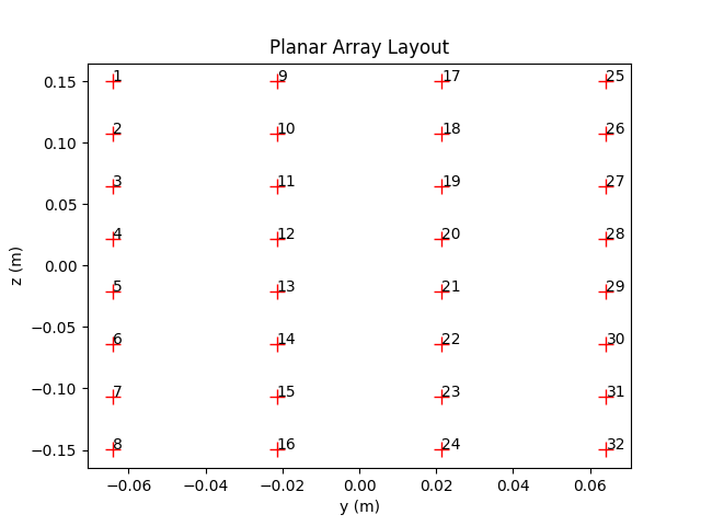
property antenna

Get/set the antenna

Type:

Antenna

property array_size

Number of antennas in the array. Dual-polarized antennas are counted as a single antenna.

Type:

int (read-only)

property num_ant

Number of linearly polarized antennas in the array. Dual-polarized antennas are counted as two linearly polarized antennas.

Type:

int (read-only)

property positions

Get/set array of relative positions \((x,y,z)\) [m] of each antenna (dual-polarized antennas are counted as a single antenna and share the same position).

Type:

[array_size, 3], tf.float

rotated_positions(orientation)

Get the antenna positions rotated according to orientation

Input:

orientation ([3], tf.float) – Orientation \((\alpha, \beta, \gamma)\) [rad] specified through three angles corresponding to a 3D rotation as defined in (3).

Output:

[array_size, 3] – Rotated positions

show()

Visualizes the antenna array

Antennas are depicted by markers that are annotated with the antenna number. The marker is not related to the polarization of an antenna.

Output:

matplotlib.pyplot.Figure – Figure depicting the antenna array

Antennas

We refer the user to the section “Far Field of a Transmitting Antenna” for various useful definitions and background on antenna modeling. An Antenna can be single- or dual-polarized and has for each polarization direction a possibly different antenna pattern.

An antenna pattern is defined as a function \(f:(\theta,\varphi)\mapsto (C_\theta(\theta, \varphi), C_\varphi(\theta, \varphi))\) that maps a pair of zenith and azimuth angles to zenith and azimuth pattern values. You can easily define your own pattern or use one of the predefined patterns below.

Transmitters (Transmitter) and receivers (Receiver) are not equipped with an Antenna but an AntennaArray that is composed of one or more antennas. All transmitters in a scene share the same AntennaArray which can be set through the scene property tx_array. The same holds for all receivers whose AntennaArray can be set through rx_array.

Antenna

class sionna.rt.Antenna(pattern, polarization=None, polarization_model=2, dtype=tf.complex64)

Class implementing an antenna

Creates an antenna object with an either predefined or custom antenna pattern. Can be single or dual polarized.

Parameters:

• pattern (str, callable, or length-2 sequence of callables) – Antenna pattern. Either one of [“iso”, “dipole”, “hw_dipole”, “tr38901”], or a callable, or a length-2 sequence of callables defining antenna patterns. In the latter case, the antenna is dual polarized and each callable defines the antenna pattern in one of the two orthogonal polarization directions. An antenna pattern is a callable that takes as inputs vectors of zenith and azimuth angles of the same length and returns for each pair the corresponding zenith and azimuth patterns.

• polarization (str or None) – Type of polarization. For single polarization, must be “V” (vertical) or “H” (horizontal). For dual polarization, must be “VH” or “cross”. Only needed if pattern is a string.

• polarization_model (int, one of [1,2]) – Polarization model to be used. Options 1 and 2 refer to polarization_model_1() and polarization_model_2(), respectively. Defaults to 2.

• dtype (tf.complex64 or tf.complex128) – Datatype used for all computations. Defaults to tf.complex64.

Example

>>> Antenna("tr38901", "VH")

property patterns

Antenna patterns for one or two polarization directions

Type:

list, callable

compute_gain

sionna.rt.antenna.compute_gain(pattern)

Computes the directivity, gain, and radiation efficiency of an antenna pattern

Given a function \(f:(\theta,\varphi)\mapsto (C_\theta(\theta, \varphi), C_\varphi(\theta, \varphi))\) describing an antenna pattern (14), this function computes the gain \(G\), directivity \(D\), and radiation efficiency \(\eta_\text{rad}=G/D\) (see (12) and text below).

Input:

pattern (callable) – A callable that takes as inputs vectors of zenith and azimuth angles of the same length and returns for each pair the corresponding zenith and azimuth patterns.

Output:

• D (float) – Directivity \(D\)

• G (float) – Gain \(G\)

• eta_rad (float) – Radiation efficiency \(\eta_\text{rad}\)

Examples

>>> compute_gain(tr38901_pattern)
(<tf.Tensor: shape=(), dtype=float32, numpy=9.606758>,
 <tf.Tensor: shape=(), dtype=float32, numpy=6.3095527>,
 <tf.Tensor: shape=(), dtype=float32, numpy=0.65678275>)

visualize

sionna.rt.antenna.visualize(pattern)

Visualizes an antenna pattern

This function visualizes an antenna pattern with the help of three figures showing the vertical and horizontal cuts as well as a three-dimensional visualization of the antenna gain.

Input:

pattern (callable) – A callable that takes as inputs vectors of zenith and azimuth angles of the same length and returns for each pair the corresponding zenith and azimuth patterns.

Output:

• matplotlib.pyplot.Figure – Vertical cut of the antenna gain

• matplotlib.pyplot.Figure – Horizontal cut of the antenna gain

• matplotlib.pyplot.Figure – 3D visualization of the antenna gain

Examples

>>> fig_v, fig_h, fig_3d = visualize(hw_dipole_pattern)

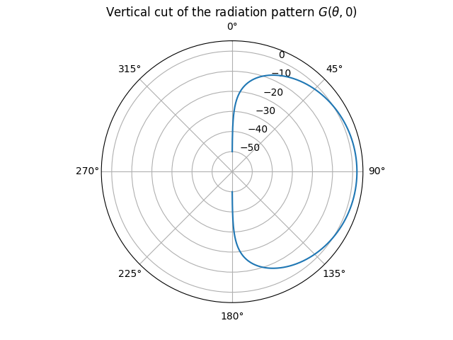
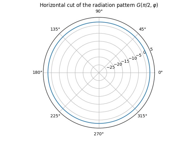
dipole_pattern

sionna.rt.antenna.dipole_pattern(theta, phi, slant_angle=0.0, polarization_model=2, dtype=tf.complex64)

Short dipole pattern with linear polarizarion (Eq. 4-26a) [Balanis97]

Input:

• theta (array_like, float) – Zenith angles wrapped within [0,pi] [rad]

• phi (array_like, float) – Azimuth angles wrapped within [-pi, pi) [rad]

• slant_angle (float) – Slant angle of the linear polarization [rad]. A slant angle of zero means vertical polarization.

• polarization_model (int, one of [1,2]) – Polarization model to be used. Options 1 and 2 refer to polarization_model_1() and polarization_model_2(), respectively. Defaults to 2.

• dtype (tf.complex64 or tf.complex128) – Datatype. Defaults to tf.complex64.

Output:

• c_theta (array_like, complex) – Zenith pattern

• c_phi (array_like, complex) – Azimuth pattern

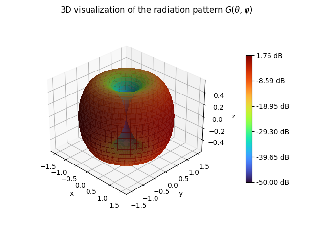
hw_dipole_pattern

sionna.rt.antenna.hw_dipole_pattern(theta, phi, slant_angle=0.0, polarization_model=2, dtype=tf.complex64)

Half-wavelength dipole pattern with linear polarizarion (Eq. 4-84) [Balanis97]

Input:

• theta (array_like, float) – Zenith angles wrapped within [0,pi] [rad]

• phi (array_like, float) – Azimuth angles wrapped within [-pi, pi) [rad]

• slant_angle (float) – Slant angle of the linear polarization [rad]. A slant angle of zero means vertical polarization.

• polarization_model (int, one of [1,2]) – Polarization model to be used. Options 1 and 2 refer to polarization_model_1() and polarization_model_2(), respectively. Defaults to 2.

• dtype (tf.complex64 or tf.complex128) – Datatype. Defaults to tf.complex64.

Output:

• c_theta (array_like, complex) – Zenith pattern

• c_phi (array_like, complex) – Azimuth pattern

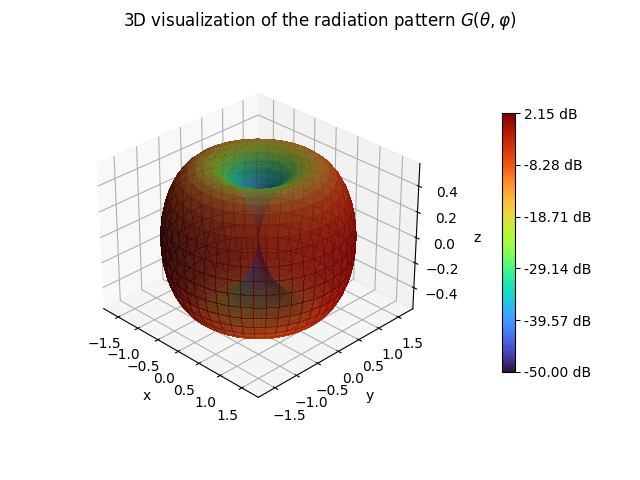
iso_pattern

sionna.rt.antenna.iso_pattern(theta, phi, slant_angle=0.0, polarization_model=2, dtype=tf.complex64)

Isotropic antenna pattern with linear polarizarion

Input:

• theta (array_like, float) – Zenith angles wrapped within [0,pi] [rad]

• phi (array_like, float) – Azimuth angles wrapped within [-pi, pi) [rad]

• slant_angle (float) – Slant angle of the linear polarization [rad]. A slant angle of zero means vertical polarization.

• polarization_model (int, one of [1,2]) – Polarization model to be used. Options 1 and 2 refer to polarization_model_1() and polarization_model_2(), respectively. Defaults to 2.

• dtype (tf.complex64 or tf.complex128) – Datatype. Defaults to tf.complex64.

Output:

• c_theta (array_like, complex) – Zenith pattern

• c_phi (array_like, complex) – Azimuth pattern

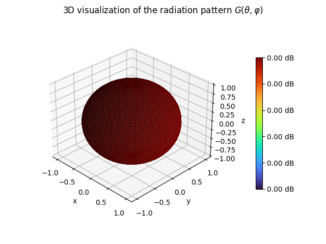
tr38901_pattern

sionna.rt.antenna.tr38901_pattern(theta, phi, slant_angle=0.0, polarization_model=2, dtype=tf.complex64)

Antenna pattern from 3GPP TR 38.901 (Table 7.3-1) [TR38901]

Input:

• theta (array_like, float) – Zenith angles wrapped within [0,pi] [rad]

• phi (array_like, float) – Azimuth angles wrapped within [-pi, pi) [rad]

• slant_angle (float) – Slant angle of the linear polarization [rad]. A slant angle of zero means vertical polarization.

• polarization_model (int, one of [1,2]) – Polarization model to be used. Options 1 and 2 refer to polarization_model_1() and polarization_model_2(), respectively. Defaults to 2.

• dtype (tf.complex64 or tf.complex128) – Datatype. Defaults to tf.complex64.

Output:

• c_theta (array_like, complex) – Zenith pattern

• c_phi (array_like, complex) – Azimuth pattern

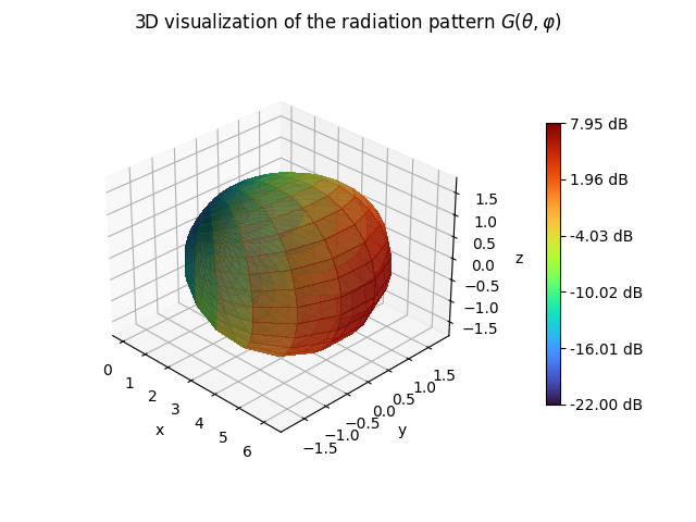
polarization_model_1

sionna.rt.antenna.polarization_model_1(c_theta, theta, phi, slant_angle)

Model-1 for polarized antennas from 3GPP TR 38.901

Transforms a vertically polarized antenna pattern \(\tilde{C}_\theta(\theta, \varphi)\) into a linearly polarized pattern whose direction is specified by a slant angle \(\zeta\). For example, \(\zeta=0\) and \(\zeta=\pi/2\) correspond to vertical and horizontal polarization, respectively, and \(\zeta=\pm \pi/4\) to a pair of cross polarized antenna elements.

The transformed antenna pattern is given by (7.3-3) [TR38901]:

\[\begin{split}\begin{align} \begin{bmatrix} C_\theta(\theta, \varphi) \\ C_\varphi(\theta, \varphi) \end{bmatrix} &= \begin{bmatrix} \cos(\psi) \\ \sin(\psi) \end{bmatrix} \tilde{C}_\theta(\theta, \varphi)\\ \cos(\psi) &= \frac{\cos(\zeta)\sin(\theta)+\sin(\zeta)\sin(\varphi)\cos(\theta)}{\sqrt{1-\left(\cos(\zeta)\cos(\theta)-\sin(\zeta)\sin(\varphi)\sin(\theta)\right)^2}} \\ \sin(\psi) &= \frac{\sin(\zeta)\cos(\varphi)}{\sqrt{1-\left(\cos(\zeta)\cos(\theta)-\sin(\zeta)\sin(\varphi)\sin(\theta)\right)^2}} \end{align}\end{split}\]

Input:

• c_tilde_theta (array_like, complex) – Zenith pattern

• theta (array_like, float) – Zenith angles wrapped within [0,pi] [rad]

• phi (array_like, float) – Azimuth angles wrapped within [-pi, pi) [rad]

• slant_angle (float) – Slant angle of the linear polarization [rad]. A slant angle of zero means vertical polarization.

Output:

• c_theta (array_like, complex) – Zenith pattern

• c_phi (array_like, complex) – Azimuth pattern

polarization_model_2

sionna.rt.antenna.polarization_model_2(c, slant_angle)

Model-2 for polarized antennas from 3GPP TR 38.901

Transforms a vertically polarized antenna pattern \(\tilde{C}_\theta(\theta, \varphi)\) into a linearly polarized pattern whose direction is specified by a slant angle \(\zeta\). For example, \(\zeta=0\) and \(\zeta=\pi/2\) correspond to vertical and horizontal polarization, respectively, and \(\zeta=\pm \pi/4\) to a pair of cross polarized antenna elements.

The transformed antenna pattern is given by (7.3-4/5) [TR38901]:

\[\begin{split}\begin{align} \begin{bmatrix} C_\theta(\theta, \varphi) \\ C_\varphi(\theta, \varphi) \end{bmatrix} &= \begin{bmatrix} \cos(\zeta) \\ \sin(\zeta) \end{bmatrix} \tilde{C}_\theta(\theta, \varphi) \end{align}\end{split}\]

Input:

• c_tilde_theta (array_like, complex) – Zenith pattern

• slant_angle (float) – Slant angle of the linear polarization [rad]. A slant angle of zero means vertical polarization.

Output:

• c_theta (array_like, complex) – Zenith pattern

• c_phi (array_like, complex) – Azimuth pattern

Reconfigurable Intelligent Surfaces (RIS)

RIS

class sionna.rt.RIS(name, position, num_rows, num_cols, num_modes=1, orientation=(0.0, 0.0, 0.0), velocity=(0.0, 0.0, 0.0), look_at=None, color=(0.862, 0.078, 0.235), dtype=tf.complex64)

Class defining a reconfigurable intelligent surface (RIS)

A RIS consists of a planar arrangement of unit cells with \(\lambda/2\) spacing. It’s PhaseProfile \(\chi_m\) and AmplitudeProfile \(A_m\) can be configured after the RIS is instantiated. Both together define the spatial modulation coefficient \(\Gamma\) which determines how the RIS reflects electro-magnetic waves.

See Reconfigurable Intelligent Surfaces (RIS) in the Primer on Electromagnetics for more details or have a look at the tutorial notebook.

An RIS instance is a callable that computes the spatial modulation coefficient and gradients/Hessians of the underlying phase profile for provided points on the RIS’ surface.

Parameters:

• name (str) – Name

• position ([3], float) – Position \((x,y,z)\) as three-dimensional vector

• num_rows (int) – Number of rows. Must at least be equal to three.

• num_cols (int) – Number of columns. Must at least be equal to three.

• num_modes (int) – Number of reradiation modes. Defaults to 1.

• orientation ([3], float) – Orientation \((\alpha, \beta, \gamma)\) specified through three angles corresponding to a 3D rotation as defined in (3). This parameter is ignored if look_at is not None. Defaults to [0,0,0]. In this case, the normal vector of the RIS points towards the positive x-axis.

• velocity ([3], float) – Velocity vector [m/s]. Used for the computation of path-specific Doppler shifts.

• look_at ([3], float | Transmitter | Receiver | RIS | Camera | None) – A position or the instance of a Transmitter, Receiver, RIS, or Camera to look at. If set to None, then orientation is used to orientate the device.

• color ([3], float) – Defines the RGB (red, green, blue) color parameter for the device as displayed in the previewer and renderer. Each RGB component must have a value within the range \(\in [0,1]\). Defaults to [0.862,0.078,0.235].

• dtype (tf.complex) – Datatype to be used in internal calculations. Defaults to tf.complex64.

Input:

• points (tf.float, [num_samples, 2]) – Tensor of 2D coordinates defining the points on the RIS at which the spatial modulation profile should be evaluated. Defaults to None. In this case, the values for all unit cells are returned.

• mode (int | None) – Reradiation mode to be considered. Defaults to None. In this case, the values for all modes are returned.

• return_grads (bool) – If True, also the first- and second-order derivatives are returned. Defaults to False.

Output:

• gamma ([num_modes, num_samples] or [num_samples], tf.complex) – Spatial modulation coefficient at the sample positions

• grads ([num_modes, num_samples, 3] or [num_samples, 3], tf.float) – Gradients of the interpolated phase profile values at the sample positions. Only returned if return_grads is True.

• hessians ([num_modes, num_samples, 3, 3] or [num_samples, 3, 3] , tf.float) – Hessians of the interpolated phase profile values at the sample positions. Only returned if return_grads is True.

property amplitude_profile

Set/get amplitude profile

Type:

AmplitudeProfile

property cell_grid

Defines the physical structure of the RIS

Type:

CellGrid

property cell_positions

Cell positions in the local coordinate system (LCS) of the RIS, ordered from top-to-bottom left-to-right.

Type:

[num_cells, 2], tf.float

property cell_world_positions

Cell positions in the global coordinate system (GCS) of the RIS, ordered from top-to-bottom left-to-right.

Type:

[num_cells, 3], tf.float

property color

Get/set the the RGB (red, green, blue) color for the device as displayed in the previewer and renderer. Each RGB component must have a value within the range \(\in [0,1]\).

Type:

[3], float

focusing_lens(sources, targets)

Configures the RIS as focusing lens

The phase profile is configured in such a way that the fields of all rays add up coherently at a specific point. In other words, the phase profile undoes the distance-based phase shift of every ray connecting a source to a target via a specific unit cell.

For a source and target at positions \(\mathbf{s}\) and \(\mathbf{t}\), the phase \(\chi_m(\mathbf{x})\) of a unit cell located at \(\mathbf{x}\) is computed as (e.g., Sec. IV-2 [Degli-Esposti22])

\[\chi_m(\mathbf{x}) = k_0 \left(\lVert\mathbf{s}-\mathbf{x}\rVert + \lVert\mathbf{s}-\mathbf{t}\rVert\right).\]

Multiple reradiation modes can be configured.

The amplitude profile is set to one everywhere with a uniform relative power allocation across modes.

Input:

• sources (tf.float, [3] or [num_modes, 3]) – Tensor defining for every reradiation mode a source from which the incoming wave originates.

• targets (tf.float, [3] or [num_modes, 3]) – Tensor defining for every reradiation mode a target towards which the incoming wave should be reflected.

look_at(target)

Sets the orientation so that the x-axis points toward a position, radio device, RIS, or camera.

Given a point \(\mathbf{x}\in\mathbb{R}^3\) with spherical angles \(\theta\) and \(\varphi\), the orientation of the radio device will be set equal to \((\varphi, \frac{\pi}{2}-\theta, 0.0)\).

Input:

target ([3], float | Transmitter | Receiver | RIS | Camera | str) – A position or the name or instance of a Transmitter, Receiver, RIS, or Camera in the scene to look at.

property name

Name

Type:

str (read-only)

property num_cells

Number of cells

Type:

int

property num_cols

Number of columns

Type:

int

property num_modes

Number of reradiation modes

Type:

int

property num_rows

Number of rows

Type:

int

property orientation

Get/set the orientation

Type:

[3], tf.float

phase_gradient_reflector(sources, targets)

Configures the RIS as ideal phase gradient reflector

For an incoming direction \(\hat{\mathbf{k}}_i\) and desired outgoing direction \(\hat{\mathbf{k}}_r\), the necessary phase gradient along the RIS with normal \(\hat{\mathbf{n}}\) can be computed as (e.g., Eq.(12) [Vitucci24]):

\[\nabla\chi_m = k_0\left( \mathbf{I}- \hat{\mathbf{n}}\hat{\mathbf{n}}^\textsf{T} \right) \left(\hat{\mathbf{k}}_i - \hat{\mathbf{k}}_r \right).\]

The phase profile is obtained by assigning zero phase to the first unit cell and evolving the other phases linearly according to the gradient across the entire RIS.

Multiple reradiation modes can be configured.

The amplitude profile is set to one everywhere with a uniform relative power allocation across modes.

Input:

• sources (tf.float, [3] or [num_modes, 3]) – Tensor defining for every reradiation mode a source from which the incoming wave originates.

• targets (tf.float, [3] or [num_modes, 3]) – Tensor defining for every reradiation mode a target towards which the incoming wave should be reflected.

property phase_profile

Set/get phase profile

Type:

PhaseProfile

property position

Get/set the position

Type:

[3], tf.float

property size

Size of the RIS (width, height) [m]

Type:

[2], tf.float

property spacing

Element spacing [m] corresponding to half a wavelength

Type:

tf.float

property velocity

Get/set the velocity vector [m/s]

Type:

[3], tf.float

property world_normal

Normal vector of the RIS in the global coordinate system (GCS)

Type:

[3], tf.float

PhaseProfile

class sionna.rt.PhaseProfile(dtype=tf.complex64)

Abstract class defining a phase profile of a RIS

A PhaseProfile instance is a callable that returns the profile values, gradients and Hessians at given points.

Parameters:

dtype (tf.complex) – Datatype to be used in internal calculations. Defaults to tf.complex64.

Input:

• points (tf.float, [num_samples, 2]) – Tensor of 2D coordinates defining the points on the RIS at which the profile should be evaluated. Defaults to None. In this case, the values for all unit cells are returned.

• mode (int | None) – Reradiation mode to be considered. Defaults to None. In this case, the values for all modes are returned.

• return_grads (bool) – If True, also the first- and second-order derivatives are returned. Defaults to False.

Output:

• values ([num_modes, num_samples] or [num_samples], tf.float) – Interpolated profile values at the sample positions

• grads ([num_modes, num_samples, 3] or [num_samples, 3], tf.float) – Gradients of the interpolated profile values at the sample positions. Only returned if return_grads is True.

• hessians ([num_modes, num_samples, 3, 3] or [num_samples, 3, 3] , tf.float) – Hessians of the interpolated profile values at the sample positions. Only returned if return_grads is True.

abstract property num_modes

Number of reradiation modes

Type:

int

DiscretePhaseProfile

class sionna.rt.DiscretePhaseProfile(cell_grid, num_modes=1, values=None, interpolator=None, dtype=tf.complex64)

Class defining a discrete phase profile of a RIS

A discrete phase profile \(\chi_m\) assigns to each of its units cells a possibly different phase value. Multiple reradiation modes can be created by super-positioning of phase profiles.

See Reconfigurable Intelligent Surfaces (RIS) in the Primer on Electromagnetics for more details.

A class instance is a callable that returns the profile values, gradients and Hessians at given points.

Parameters:

• cell_grid (CellGrid) – Defines the physical structure of the RIS

• num_modes (int) – Number of reradiation modes. Defaults to 1.

• values (tf.float or tf.Variable, [num_modes, num_rows, num_cols]) – Phase values [rad] for each reradiation mode and unit cell. num_rows and num_cols are defined by the cell_grid. Defaults to None.

• interpolator (ProfileInterpolator) – Determines how the discrete values of the profile are interpolated to a continuous profile which is defined at any point on the RIS. Defaults to None. In this case, the LagrangeProfileInterpolator will be used.

• dtype (tf.complex) – Datatype to be used in internal calculations. Defaults to tf.complex64.

Input:

• points (tf.float, [num_samples, 2]) – Tensor of 2D coordinates defining the points on the RIS at which the profile should be evaluated. Defaults to None. In this case, the values for all unit cells are returned.

• mode (int | None) – Reradiation mode to be considered. Defaults to None. In this case, the values for all modes are returned.

• return_grads (bool) – If True, also the first- and second-order derivatives are returned. Defaults to False.

Output:

• values ([num_modes, num_samples] or [num_samples], tf.float) – Interpolated profile values at the sample positions

• grads ([num_modes, num_samples, 3] or [num_samples, 3], tf.float) – Gradients of the interpolated profile values at the sample positions. Only returned if return_grads is True.

• hessians ([num_modes, num_samples, 3, 3] or [num_samples, 3, 3] , tf.float) – Hessians of the interpolated profile values at the sample positions. Only returned if return_grads is True.

property cell_grid

Defines the physical structure of the RIS

Type:

CellGrid

property num_modes

Number of reradiation modes

Type:

int

property shape

Shape of the tensor holding the values of the discrete profile

Type:

tf.TensorShape

show(mode=0)

Visualizes the profile as a 3D plot

Input:

mode (int | None) – Reradation mode to be shown. Defaults to 0.

Output:

matplotlib.pyplot.Figure – 3D plot of the profile

property spacing

Element spacing [m] corresponding to half a wavelength

Type:

tf.float

property values

Set/get the discrete values of the profile for each reradiation mode

Type:

[shape], tf.float

AmplitudeProfile

class sionna.rt.AmplitudeProfile(dtype=tf.complex64)

Abstract class defining an amplitude profile of a RIS

An AmplitudeProfile instance is a callable that returns the profile values, gradients and Hessians at given points.

Parameters:

dtype (tf.complex) – Datatype to be used in internal calculations. Defaults to tf.complex64.

Input:

• points (tf.float, [num_samples, 2]) – Tensor of 2D coordinates defining the points on the RIS at which the profile should be evaluated. Defaults to None. In this case, the values for all unit cells are returned.

• mode (int | None) – Reradiation mode to be considered. Defaults to None. In this case, the values for all modes are returned.

• return_grads (bool) – If True, also the first- and second-order derivatives are returned. Defaults to False.

Output:

• values ([num_modes, num_samples] or [num_samples], tf.float) – Interpolated profile values at the sample positions

• grads ([num_modes, num_samples, 3] or [num_samples, 3], tf.float) – Gradients of the interpolated profile values at the sample positions. Only returned if return_grads is True.

• hessians ([num_modes, num_samples, 3, 3] or [num_samples, 3, 3] , tf.float) – Hessians of the interpolated profile values at the sample positions. Only returned if return_grads is True.

abstract property mode_powers

Relative power of reradiation modes

Type:

[num_modes], tf.float

abstract property num_modes

Number of reradiation modes

Type:

int

DiscreteAmplitudeProfile

class sionna.rt.DiscreteAmplitudeProfile(cell_grid, num_modes=1, values=None, mode_powers=None, interpolator=None, dtype=tf.complex64)

Class defining a discrete amplitude profile of a RIS

A discrete amplitude profile \(A_m\) assigns to each of its units cells a possibly different amplitude value. Multiple reradiation modes can be obtained by super-positioning of profiles. The relative power of reradiation modes can be controlled via the reradiation coefficients \(p_m\).

See Reconfigurable Intelligent Surfaces (RIS) for more details.

A class instance is a callable that returns the profile values, gradients and Hessians at given points.

Parameters:

• cell_grid (CellGrid) – Defines the physical structure of the RIS

• num_modes (int) – Number of reradiation modes. Defaults to 1.

• values (tf.float or tf.Variable, [num_modes, num_rows, num_cols]) – Amplitude values for each reradiation mode and unit cell. num_rows and num_cols are defined by the cell_grid. Defaults to None.

• mode_powers (tf.float, [num_modes]) – Relative powers or reradition coefficients of reradiation modes. Defaults to None. In this case, all reradiation modes get an equal fraction of the total power.

• interpolator (ProfileInterpolator) – Determines how the discrete values of the profile are interpolated to a continuous profile which is defined at any point on the RIS. Defaults to None. In this case, the LagrangeProfileInterpolator will be used.

• dtype (tf.complex) – Datatype to be used in internal calculations. Defaults to tf.complex64.

Input:

• points (tf.float, [num_samples, 2]) – Tensor of 2D coordinates defining the points on the RIS at which the profile should be evaluated. Defaults to None. In this case, the values for all unit cells are returned.

• mode (int | None) – Reradiation mode to be considered. Defaults to None. In this case, the values for all modes are returned.

• return_grads (bool) – If True, also the first- and second-order derivatives are returned. Defaults to False.

Output:

• values ([num_modes, num_samples] or [num_samples], tf.float) – Interpolated profile values at the sample positions

• grads ([num_modes, num_samples, 3] or [num_samples, 3], tf.float) – Gradients of the interpolated profile values at the sample positions. Only returned if return_grads is True.

• hessians ([num_modes, num_samples, 3, 3] or [num_samples, 3, 3] , tf.float) – Hessians of the interpolated profile values at the sample positions. Only returned if return_grads is True.

property cell_grid

Defines the physical structure of the RIS

Type:

CellGrid

property mode_powers

Relative power of reradiation modes

Type:

[num_modes], tf.float

property num_modes

Number of reradiation modes

Type:

int

property shape

Shape of the tensor holding the values of the discrete profile

Type:

tf.TensorShape

show(mode=0)

Visualizes the profile as a 3D plot

Input:

mode (int | None) – Reradation mode to be shown. Defaults to 0.

Output:

matplotlib.pyplot.Figure – 3D plot of the profile

property spacing

Element spacing [m] corresponding to half a wavelength

Type:

tf.float

property values

Set/get the discrete values of the profile for each reradiation mode

Type:

[shape], tf.float

ProfileInterpolator

class sionna.rt.ProfileInterpolator(discrete_profile)

Abstract class defining an interpolator of a discrete profile

A ProfileInterpolator instance is a callable that interpolate the discrete profile to specified points. Optionally, the gradients and Hessians are returned.

Parameters:

discrete_profile (DiscreteProfile) – Discrete profile to be interpolated

Input:

• points ([num_samples, 2], tf.float) – Positions at which to interpolate the profile

• mode (int | None) – Mode of the profile to interpolate. If None. all modes are interpolated. Defaults to None.

• return_grads (bool) – If True, gradients and Hessians are computed. Defaults to False.

Output:

• values ([num_modes, num_samples] or [num_samples], tf.float) – Interpolated profile values at the sample positions

• grads ([num_modes, num_samples, 3] or [num_samples, 3], tf.float) – Gradients of the interpolated profile values at the sample positions

• hessians ([num_modes, num_samples, 3, 3] or [num_samples,3,3], tf.float) – Hessians of the interpolated profile values at the sample positions

property spacing

Element spacing [m] corresponding to half a wavelength

Type:

tf.float

LagrangeProfileInterpolator

class sionna.rt.LagrangeProfileInterpolator(discrete_profile)

Class defining a ProfileInterpolator using Lagrange polynomials

The class instance is a callable that interpolates a discrete profile at arbitrary positions using two-dimensional 2nd-order Lagrange interpolation.

A discrete profile \(P(y_i,z_j)\in\mathbb{R}\) defined on a grid of points \(y_i,z_j\) for \(i,j \in [1,2,3]\) is interpolated to position \(y,z\) as

\[\begin{align} P(y,z) &= \sum_{i,j} P(y_i,z_j) \ell_{i,y}(y) \ell_{j,z}(z) \end{align}\]

where \(\ell_{i,y}(y)\), \(\ell_{j,z}(z)\) are the one-dimensional 2nd-order Lagrange polynomials, defined as

\[\begin{split}\begin{align} \ell_{i,y}(y) &= \prod_{j \ne i} \frac{y-y_j}{y_i-y_j} \\ \ell_{j,z}(z) &= \prod_{i \ne j} \frac{z-z_i}{z_j-z_i}. \end{align}\end{split}\]

Note that the formulation above assumes for simplicity only a 3x3 grid of points. However, the implementation finds for every position the closest 3x3 grid points of the discrete profile which are used for interpolation.

In order to compute spatial gradients and Hessians, we extend the the profile with a dummy \(x\) dimension, i.e., \(P(x,y,z)=P(y,z)\), such that

\[\begin{split}\begin{align} \nabla P(x,y,z) &= \begin{bmatrix} 0, \frac{\partial P(x,y,z)}{\partial y}, \frac{\partial P(x,y,z)}{\partial z} \end{bmatrix}^{\textsf{T}}\\ H_P(x,y,z) &= \begin{bmatrix} 0 & 0 & 0 \\ 0 & \frac{\partial^2 P(x,y,z)}{\partial y^2} & \frac{\partial^2 P(x,y,z)}{\partial y \partial z} \\ 0 & \frac{\partial^2 P(x,y,z)}{\partial z \partial y} & \frac{\partial^2 P(x,y,z)}{\partial z^2} \end{bmatrix} \end{align}.\end{split}\]

Parameters:

discrete_profile (DiscreteProfile) – Discrete profile to be interpolated

Input:

• points ([num_samples, 2], tf.float) – Positions at which to interpolate the profile

• mode (int | None) – Mode of the profile to interpolate. If None, all modes are interpolated. Defaults to None.

• return_grads (bool) – If True, gradients and Hessians are computed. Defaults to False.

Output:

• values ([num_modes, num_samples] or [num_samples], tf.float) – Interpolated profile values at the sample positions

• grads ([num_modes, num_samples, 3] or [num_samples, 3], tf.float) – Gradients of the interpolated profile values at the sample positions

• hessians ([num_modes, num_samples, 3, 3] or [num_samples, 3, 3] , tf.float) – Hessians of the interpolated profile values at the sample positions

static lagrange_polynomials(x, x_i, return_derivatives=True)

Compute the 2nd-order Lagrange polynomials

Optionally, the first- and second-order derivatives are returned.

The 2nd-order Lagrange polynomials \(\ell_j(x)\), \(j=1,2,3\), for position \(x\in\mathbb{R}\) are computed using three distinct support positions \(x_i\) for \(i=1,2,3\):

\[\begin{split}\begin{align} \ell_j(x) &= \prod_{\substack{1\leq i \leq 3 \\ i \ne j}} \frac{x-x_i}{x_j-x_i}. \end{align}\end{split}\]

Their first- and second-order derivatives are then respectively given as

\[\begin{split}\begin{align} \ell'_j(x) &= \left(\sum_{i \ne j} x-x_i\right) \left(\prod_{i \ne j} x_j-x_i\right)^{-1} \\ \ell''_j(x) &= 2 \left(\prod_{i \ne j} x_j-x_i\right)^{-1}. \end{align}\end{split}\]

Input:

• x ([batch_size], tf.float) – Sample positions

• x_i ([batch_size, 3], tf.float) – Support positions for every sample position

• return_derivatives (bool) – If True, also the first- and second-order derivatives of the Lagrange polynomials are returned. Defaults to True.

Output:

• l_i ([batch_size, 3], tf.float) – Lagrange polynomials for each sample position

• deriv_1st ([batch_size, 3], tf.float) – First-order derivatives for each sample position. Only returned if return_derivatives is True.

• deriv_2nd ([batch_size, 3], tf.float) – Second-order derivatives for each sample position. Only returned if return_derivatives is True.

property spacing

Element spacing [m] corresponding to half a wavelength

Type:

tf.float

CellGrid

class sionna.rt.CellGrid(num_rows, num_cols, dtype=tf.complex64)

Class defining a cell grid that determines the physical structure of a RIS

The cell grid specifies the location of unit cells within the y-z plane assuming a homogenous spacing of 0.5. The actual positions are computed by multiplying the cell positions by the wavelength and rotating them according to the RIS’ orientation.

A cell grid must have at least three columns and rows to ensure that discrete phase and amplitude profiles of the RIS can be interpolated.

Parameters:

• num_rows (int) – Number of rows. Must at least be equal to three.

• num_cols (int) – Number of columns. Must at least be equal to three.

• dtype (tf.complex) – Datatype to be used in internal calculations. Defaults to tf.complex64.

property cell_positions

Cell positions ordered from top-to-bottom left-to-right

Type:

[num_cells, 2], tf.float

property cell_y_positions

y-coordinates of cells ordered from left-to-right

Type:

[num_cols], tf.float

property cell_z_positions

z-coordinates of cells ordered from top-to-bottom

Type:

[num_rows], tf.float

property num_cells

Number of cells

Type:

int

property num_cols

Number of columns

Type:

int

property num_rows

Number of rows

Type:

int

Utility Functions

cross

sionna.rt.cross(u, v)

Computes the cross (or vector) product between u and v

Input:

• u ([…,3]) – First vector

• v ([…,3]) – Second vector

Output:

[…,3] – Cross product between u and v

dot

sionna.rt.dot(u, v, keepdim=False, clip=False)

Computes and the dot (or scalar) product between u and v

Input:

• u ([…,3]) – First vector

• v ([…,3]) – Second vector

• keepdim (bool) – If True, keep the last dimension. Defaults to False.

• clip (bool) – If True, clip output to [-1,1]. Defaults to False.

Output:

[…,1] or […] – Dot product between u and v. The last dimension is removed if keepdim is set to False.

outer

sionna.rt.outer(u, v)

Computes the outer product between u and v

Input:

• u ([…,3]) – First vector

• v ([…,3]) – Second vector

Output:

[…,3,3] – Outer product between u and v

normalize

sionna.rt.normalize(v)

Normalizes v to unit norm

Input:

v ([…,3], tf.float) – Vector

Output:

• […,3], tf.float – Normalized vector

• […], tf.float – Norm of the unnormalized vector

phi_hat

sionna.rt.phi_hat(phi)

Computes the spherical unit vector \(\hat{\boldsymbol{\varphi}}(\theta, \varphi)\) as defined in (1)

Input:

phi (same shape as theta, tf.float) – Azimuth angles \(\varphi\) [rad]

Output:

theta_hat (phi.shape + [3], tf.float) – Vector \(\hat{\boldsymbol{\varphi}}(\theta, \varphi)\)

rotate

sionna.rt.rotate(p, angles, inverse=False)

Rotates points p by the angles according to the 3D rotation defined in (3)

Input:

• p ([…,3], tf.float) – Points to rotate

• angles ([…, 3]) – Angles for the rotations [rad]. The last dimension corresponds to the angles \((\alpha,\beta,\gamma)\) that define rotations about the axes \((z, y, x)\), respectively.

• inverse (bool) – If True, the inverse rotation is applied, i.e., the transpose of the rotation matrix is used. Defaults to False

Output:

[…,3] – Rotated points p

rotation_matrix

sionna.rt.rotation_matrix(angles)

Computes rotation matrices as defined in (3)

The closed-form expression in (7.1-4) [TR38901] is used.

Input:

angles ([…,3], tf.float) – Angles for the rotations [rad]. The last dimension corresponds to the angles \((\alpha,\beta,\gamma)\) that define rotations about the axes \((z, y, x)\), respectively.

Output:

[…,3,3], tf.float – Rotation matrices

rot_mat_from_unit_vecs

sionna.rt.rot_mat_from_unit_vecs(a, b)

Computes Rodrigues` rotation formula (6)

Input:

• a ([…,3], tf.float) – First unit vector

• b ([…,3], tf.float) – Second unit vector

Output:

[…,3,3], tf.float – Rodrigues’ rotation matrix

r_hat

sionna.rt.r_hat(theta, phi)

Computes the spherical unit vetor \(\hat{\mathbf{r}}(\theta, \phi)\) as defined in (1)

Input:

• theta (arbitrary shape, tf.float) – Zenith angles \(\theta\) [rad]

• phi (same shape as theta, tf.float) – Azimuth angles \(\varphi\) [rad]

Output:

rho_hat (phi.shape + [3], tf.float) – Vector \(\hat{\mathbf{r}}(\theta, \phi)\) on unit sphere

sample_points_on_hemisphere

sionna.rt.sample_points_on_hemisphere(normals, num_samples=1)

Randomly sample points on hemispheres defined by their normal vectors

Input:

• normals ([batch_size, 3], tf.float) – Normal vectors defining hemispheres

• num_samples (int) – Number of random samples to draw for each hemisphere defined by its normal vector. Defaults to 1.

Output:

points ([batch_size, num_samples, 3], tf.float or [batch_size, 3], tf.float if num_samples=1.) – Random points on the hemispheres

theta_hat

sionna.rt.theta_hat(theta, phi)

Computes the spherical unit vector \(\hat{\boldsymbol{\theta}}(\theta, \varphi)\) as defined in (1)

Input:

• theta (arbitrary shape, tf.float) – Zenith angles \(\theta\) [rad]

• phi (same shape as theta, tf.float) – Azimuth angles \(\varphi\) [rad]

Output:

theta_hat (phi.shape + [3], tf.float) – Vector \(\hat{\boldsymbol{\theta}}(\theta, \varphi)\)

theta_phi_from_unit_vec

sionna.rt.theta_phi_from_unit_vec(v)

Computes zenith and azimuth angles (\(\theta,\varphi\)) from unit-norm vectors as described in (2)

Input:

v ([…,3], tf.float) – Tensor with unit-norm vectors in the last dimension

Output:

• theta ([…], tf.float) – Zenith angles \(\theta\)

• phi ([…], tf.float) – Azimuth angles \(\varphi\)

watt_to_dbm

sionna.rt.watt_to_dbm(power)

Converts \(P_{W}\) [W] to \(P_{dBm}\) [dBm] via the formula: \(P_{dBm} = 30 + 10 \log_{10}(P_W)\)

Input:

power (float) – Power [W]

Output:

float – Power [dBm]

dbm_to_watt

sionna.rt.dbm_to_watt(dbm)

Converts dBm to Watt via the formula: \(P_W = 10^{\frac{P_{dBm}-30}{10}}\)

Input:

dbm (float) – Power [dBm]

Output:

float – Power [W]

References:

[Balanis97] (1,2)

A. Balanis, “Antenna Theory: Analysis and Design,” 2nd Edition, John Wiley & Sons, 1997.

[ITUR_P2040_2] (1,2)

ITU-R, “Effects of building materials and structures on radiowave propagation above about 100 MHz“, Recommendation ITU-R P.2040-2

[SurfaceIntegral]

Wikipedia, “Surface integral”, accessed Jun. 22, 2023.

[Wiffen2018]

F. Wiffen et al., “Comparison of OTFS and OFDM in Ray Launched sub-6 GHz and mmWave Line-of-Sight Mobility Channels”, Proc. IEEE Int. Sym. Personal, Indoor and Mobil Radio Commun. (PIMRC), Bologna, Italy, Sep. 2018.