Optical Channel with Lumped Amplification
In this notebook, you will learn how to simulate the transmission of a single Gaussian impulse over a lumped amplification channel model consisting of multiple fiber spans and optical amplifiers, so-called Erbium Doped Fiber Amplifiers (EDFA), as shown in the Figure below. We assume a standard single mode fiber (S-SMF) and denote the fiber length between two amplifiers by \(\ell_\text{span}\).

Let \(G\) denote the amplifier gain and \(F\) the noise figure of each EDFA.
As we focus on the optical channel and not the corresponding signal processing, the transmitter directly generates the optical signal. Hence, all components that, in practice, are required to generate the optical signal given an electrical control voltage (e.g., the Mach-Zehnder-Modulator (MZM)) are assumed to be ideal or are neglected. The same holds on the receiver side, where the photodiode that would add shot noise is neglected.
To provide a better understanding of the implemented channel impairments (attenuation, noise, dispersion, nonlinearity) introduced during propagation, those are successively enabled, starting with attenuation.
Table of Contents
Setup
[1]:
import os
if os.getenv("CUDA_VISIBLE_DEVICES") is None:
    gpu_num = 0 # Use "" to use the CPU
    os.environ["CUDA_VISIBLE_DEVICES"] = f"{gpu_num}"
os.environ['TF_CPP_MIN_LOG_LEVEL'] = '3'

# Import Sionna
try:
    import sionna
except ImportError as e:
    # Install Sionna if package is not already installed
    import os
    os.system("pip install sionna")
    import sionna

import tensorflow as tf
# Configure the notebook to use only a single GPU and allocate only as much memory as needed
# For more details, see https://www.tensorflow.org/guide/gpu
gpus = tf.config.list_physical_devices('GPU')
if gpus:
    try:
        tf.config.experimental.set_memory_growth(gpus[0], True)
    except RuntimeError as e:
        print(e)
# Avoid warnings from TensorFlow
tf.get_logger().setLevel('ERROR')

# Set random seed for reproducibility
sionna.config.seed = 42
from sionna.channel import utils

import numpy as np
%matplotlib inline
import matplotlib.pyplot as plt
Impulse Generation
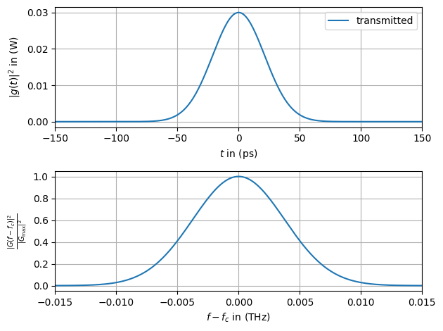
Before diving into the first channel model, the simulation shall be parametrized and the initial Gaussian impulse
is generated. The impulse shall have peak power \(P_0\) and a pulse duration of \(T_0\). Note that the Gaussian filter is infinitely long, such that \(T_0\) is the full width at half-maximum (FWHM) pulse duration.
Further, the simulation window is set to \(T_\mathrm{sim}=1000\,\mathrm{ps}\) and the sample duration is set to \(\Delta_t=1\,\mathrm{ps}\).
[2]:
# Simulation parameters
dtype = tf.complex128  # Simulation accuracy (double)
t_sim = int(1e4)  # (ps) Simulation time window
n_sim = int(1e4)  # Number of simulation samples

# Channel parameters
n_span = 3

# Impulse parameters
p_0 = 3e-2  # (W) Peak power of the Gaussian pulse
t_0 = 50  # (ps) Norm. temporal scaling of the Gaussian pulse

# Support
dt = t_sim / n_sim  # (s) sample duration
t, f = utils.time_frequency_vector(
    n_sim, dt, dtype=dtype.real_dtype)  # (ps), (THz) Time and frequency vector

# Generate Gaussian impulse
g_0 = np.sqrt(p_0 * 2**(-((2.0*t / t_0) ** 2.0)))
g_0 = tf.cast(g_0, dtype=dtype)
G_0 = tf.signal.fftshift(
        tf.abs(
            tf.cast(dt, dtype) *
            tf.signal.fft(g_0) /
            tf.cast(tf.math.sqrt(2 * np.pi), dtype)
        ) ** 2
)
[3]:
fig, (ax1, ax2) = plt.subplots(2, 1)

ax1.plot(t.numpy().flatten(), np.abs(g_0.numpy().flatten())**2, '-')
ax1.set_xlim(-150, 150)
ax1.set_xlabel(r"$t$ in (ps)")
ax1.set_ylabel(r"$|g(t)|^2$ in (W)")
ax1.grid()

ax2.plot(
    f.numpy().flatten(),
    (G_0.numpy().flatten())/np.max(G_0.numpy().flatten()),
    '-')
ax2.set_xlim(-0.015, 0.015)
ax2.set_xlabel(r"$f-f_c$ in (THz)")
ax2.set_ylabel(r"$\frac{|G(f-f_c)|^2}{|G_\mathrm{max}|^2}$")
ax2.grid()

ax1.legend(['transmitted'])
plt.tight_layout()
plt.show()
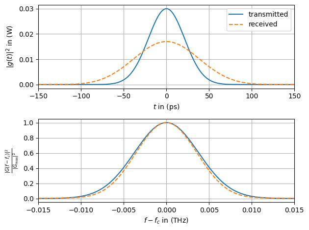
Attenuation
Attenuation is present in all media including optical fibers. A typical value of \(\alpha=0.046\,\mathrm{km}^{-1}\) is used in this notebook. To compensate for this, Erbium doped fiber amplifiers (EDFAs) are required, as shown in the figure at the beginning of this notebook.
Amplified Spontaneous Emission Noise
An optical channel model contains several sources of noise, e.g., amplified spontaneous emission (ASE) and Rayleigh scattering. However, for this experiment, only ASE noise is implemented. It was shown in [1] that this is the most dominant source of noise.
As we assume a discrete lumped amplification, ASE noise is introduced only due to the amplification by the EDFAs. The noise power is given as
and, hence, depends on the gain \(G\), the (linear) noise figure \(F\), the carrier frequency \(f_\text{c}\), and the simulation bandwidth \(f_\mathrm{sim}\). The intermediate quantitiy \(\rho_\mathrm{ASE}\) denotes the noise spectral density of the EDFAs and \(h\) is Planck’s constant. Usually, not the simulation bandwidth but the captured bandwidth \(W\) of the receiver is used. Here, for demonstration purpose, our receiver has an infinite bandwidth that is only limited by the simulation \(W=f_\mathrm{sim}\).
Note that Sionna also provides ideally distributed Raman amplification, where the noise is introduced in a fiber span. This can be enabled by setting with_amplification to True when instantiating the SSFM layer.
Channel Configuration
The fiber (i.e., SSFM) is implemented using normalized units for distance and time. Hence, it is required that the units of the same kind (time, distance, power) for all parameters (\(\alpha\), \(\beta_2\), …) have to be given with the same unit prefix, e.g., for time use always \(\mathrm{ps}\). This does not only simplify the usage of the SSFM but also prevents from dealing with different orders of magnitude within the SSFM.
For our first experiment only ASE noise is considered and, thus, nonlinearity and chromatic dispersion (CD) are disabled. Attenuation is kept enabled such that the amplifiers are required and introduce the noise. The gain is chosen such that the link becomes transparent (input power equals output power).
[4]:
# Normalization
t_norm = 1e-12  # (s) -> (ps) Time normalization
z_norm = 1e3  # (m) -> (km) Distance normalization

# Fiber parameters
f_c = 193.55e12  # (Hz) Abs. Carrier frequency
length_sp = 80.0  # (km) Norm. fiber span length
alpha = 0.046  # (1/km) Norm. fiber attenuation

# EDFA parameters
g_edfa = tf.exp(alpha * length_sp)
f_edfa = 10**(5/10)  # (1) Noise figure
[5]:
span = sionna.channel.optical.SSFM(
            alpha=alpha,
            f_c=f_c,
            length=length_sp,
            sample_duration=dt,
            with_amplification=False,
            with_attenuation=True,
            with_dispersion=False,
            with_nonlinearity=False,
            dtype=dtype,
            t_norm=t_norm)

amplifier = sionna.channel.optical.EDFA(
            g=g_edfa,
            f=f_edfa,
            f_c=f_c,
            dt=dt * t_norm,  # t_norm is in absolute (not normalized) units
            dtype=dtype)

def lumped_amplification_channel(inputs):
    (u_0) = inputs

    u = u_0
    for _ in range(n_span):
        u = span(u)
        u = amplifier(u)

    return u
Transmission
Next, the impulse is transmitted over the channel and the output is visualized.
[6]:
x = g_0
y = lumped_amplification_channel(x)

X = tf.signal.fftshift(
    tf.abs(
        tf.cast(dt, dtype) *
        tf.signal.fft(x) /
        tf.cast(tf.math.sqrt(2 * np.pi), dtype)
    ) ** 2
)

Y = tf.signal.fftshift(
    tf.abs(
        tf.cast(dt, dtype) *
        tf.signal.fft(y) /
        tf.cast(tf.math.sqrt(2 * np.pi), dtype)
    ) ** 2
)
[7]:
fig, (ax1, ax2) = plt.subplots(2, 1)

ax1.plot(t.numpy().flatten(), np.abs(x.numpy().flatten())**2, '-')
ax1.plot(t.numpy().flatten(), np.abs(y.numpy().flatten())**2, '--')
ax1.set_xlim(-150, 150)
ax1.set_xlabel(r"$t$ in (ps)")
ax1.set_ylabel(r"$|g(t)|^2$ in (W)")
ax1.grid()

ax2.plot(
    f.numpy().flatten(),
    (X.numpy().flatten())/np.max(X.numpy().flatten()),
    '-')
ax2.plot(
    f.numpy().flatten(),
    (Y.numpy().flatten())/np.max(Y.numpy().flatten()),
    '--')
ax2.set_xlim(-0.015, 0.015)
ax2.set_xlabel(r"$f-f_c$ in (THz)")
ax2.set_ylabel(r"$\frac{|G(f-f_c)|^2}{|G_\mathrm{max}|^2}$")
ax2.grid()

ax1.legend(['transmitted', 'received'])
plt.tight_layout()

plt.show()
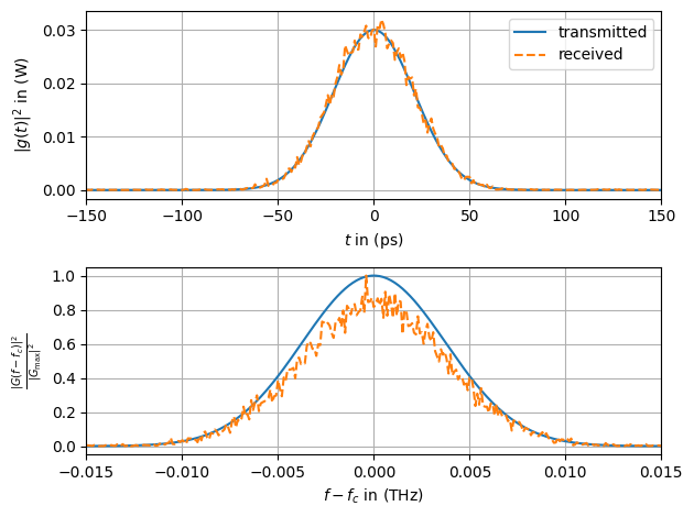
As can be seen, attenuation is completely compensated by the EDFAs. However, they introduce significant noise.
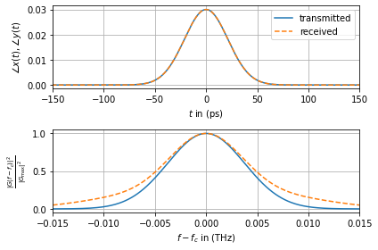
Chromatic Dispersion
After having seen how the noise distorts the original Gaussian impulse, we can now enable the next linear effect, which is chromatic dispersion (CD). Regarding the nonlinear Schrödinger equation that describes the propagation of an optical signal, the impact of CD is parametrized by the group velocity dispersion (GVD) parameter \(\beta_2\), where \(\beta_2=-21.67\,\mathrm{ps}^2\mathrm{km}^{-1}\) is a typical choice.
Channel Configuration
Besides the present parameters we now set \(\beta_2\). For a better understanding of CD we disable the noise (EDFA.f = 0) from the previous section.
[8]:
beta_2 = -21.67 # (ps^2/km) Norm. group velocity dispersion
[9]:
span_cd = sionna.channel.optical.SSFM(
            alpha=alpha,
            beta_2=beta_2,
            f_c=f_c,
            length=length_sp,
            sample_duration=dt,
            with_amplification=False,
            with_attenuation=True,
            with_dispersion=True,
            with_nonlinearity=False,
            dtype=dtype,
            t_norm=t_norm)

amplifier_cd = sionna.channel.optical.EDFA(
            g=g_edfa,
            f=0,
            f_c=f_c,
            dt=dt * t_norm,
            dtype=dtype)


def lumped_amplification_channel_cd(inputs):
    (u_0) = inputs

    u = u_0
    for _ in range(n_span):
        u = span_cd(u)
        u = amplifier_cd(u)

    return u
Transmission
We now transmit the previously generated Gaussian impulse over the optical fiber and compare the received signal with the transmitted impulse.
[10]:
x = g_0  # previously generated Gaussian impulse
y = lumped_amplification_channel_cd(x)

X = tf.signal.fftshift(
    tf.abs(
        tf.cast(dt, dtype) *
        tf.signal.fft(x) /
        tf.cast(tf.math.sqrt(2 * np.pi), dtype)
    ) ** 2
)

Y = tf.signal.fftshift(
    tf.abs(
        tf.cast(dt, dtype) *
        tf.signal.fft(y) /
        tf.cast(tf.math.sqrt(2 * np.pi), dtype)
    ) ** 2
)

X_angle = tf.math.angle(tf.signal.fftshift(tf.signal.fft(x)))
Y_angle = tf.math.angle(tf.signal.fftshift(tf.signal.fft(y)))
[11]:
fig, (ax1, ax2) = plt.subplots(2, 1)

ax1.plot(t.numpy().flatten(), np.abs(x.numpy().flatten())**2, '-')
ax1.plot(t.numpy().flatten(), np.abs(y.numpy().flatten())**2, '--')
ax1.set_xlim(-250, 250)
ax1.set_xlabel(r"$t$ in (ps)")
ax1.set_ylabel(r"$|g(t)|^2$ in (W)")
ax1.grid()

ax2.plot(
    f.numpy().flatten(),
    (X.numpy().flatten())/np.max(X.numpy().flatten()),
    '-')
ax2.plot(
    f.numpy().flatten(),
    (Y.numpy().flatten())/np.max(Y.numpy().flatten()),
    '--')
ax2.set_xlim(-0.015, 0.015)
ax2.set_xlabel(r"$f-f_c$ in (THz)")
ax2.set_ylabel(r"$\frac{|G(f-f_c)|^2}{|G_\mathrm{max}|^2}$")
ax2.grid()

ax1.legend(['transmitted', 'received'])
plt.tight_layout()

plt.show()
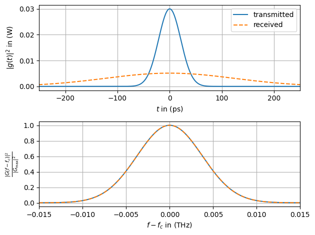
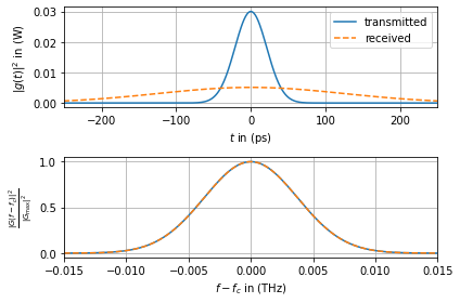
Compared to the transmit impulse the received one has significantly broadened in time. The absolute value of the spectrum, nevertheless, stayed the same. By plotting the phase of the received signal one can see the typical parabolic shift.
[12]:
fig, (ax1) = plt.subplots(1, 1, tight_layout=True)

ax1.plot(t.numpy().flatten(), np.angle(x.numpy().flatten()), '-')
ax1.plot(t.numpy().flatten(), np.angle(y.numpy().flatten()), '--')
ax1.set_xlim(-750, 750)
ax1.set_xlabel(r"$t$ in (ps)")
ax1.set_ylabel("$\u2220 x(t), \u2220 y(t)$")
ax1.grid()

ax1.legend(['transmitted', 'received'])
plt.tight_layout()

plt.show()
Kerr Nonlinearity
Last, we depict the Kerr nonlinearity and, for a better understanding, disable all previous impairments. This nonlinear effect applies a phase shift to the transmitted signal depending on its instantaneous power. Hence, we should see a phase that, in contrast to the phase of the original signal which is zero, follows the (inverse) absolute value of the impulse.
Note: Only the interaction between Kerr nonlinearity and CD requires an SSFM for fiber simulation. Otherwise (as done so far), the transfer function of the individual effect is just a single multiplication (in time- or Fourier-domain, respectively).
Channel configuration
Similarly to the definition of CD, we specify a typical value for \(\gamma=1.27\,\mathrm{\frac{1}{km W}}\).
[13]:
gamma = 1.27 # (1/W/km) Nonlinearity coefficient
[14]:
span_nl = sionna.channel.optical.SSFM(
            alpha=alpha,
            beta_2=beta_2,
            f_c=f_c,
            length=length_sp,
            sample_duration=dt,
            with_amplification=False,
            with_attenuation=True,
            with_dispersion=False,
            with_nonlinearity=True,
            dtype=dtype, t_norm=t_norm)

amplifier_nl = sionna.channel.optical.EDFA(
            g=g_edfa,
            f=0,
            f_c=f_c,
            dt=dt * t_norm,
            dtype=dtype)


def lumped_amplification_channel_nl(inputs):
    (u_0) = inputs

    u = u_0
    for _ in range(n_span):
        u = span_nl(u)
        u = amplifier_nl(u)

    return u
Transmission
We now transmit the same Gaussian impulse again over the optical fiber where only Kerr nonlinearity is activated.
[15]:
x = g_0
y = lumped_amplification_channel_nl(x)

X = tf.signal.fftshift(
    tf.abs(
        tf.cast(dt, dtype) *
        tf.signal.fft(x) /
        tf.cast(tf.math.sqrt(2 * np.pi), dtype)
    ) ** 2
)

Y = tf.signal.fftshift(
    tf.abs(
        tf.cast(dt, dtype) *
        tf.signal.fft(y) /
        tf.cast(tf.math.sqrt(2 * np.pi), dtype)
    ) ** 2
)

X_angle = tf.math.angle(tf.signal.fftshift(tf.signal.fft(x)))
Y_angle = tf.math.angle(tf.signal.fftshift(tf.signal.fft(y)))
[16]:
fig, (ax1, ax2) = plt.subplots(2, 1)

ax1.plot(t.numpy().flatten(), np.abs(x.numpy().flatten())**2, '-')
ax1.plot(t.numpy().flatten(), np.abs(y.numpy().flatten())**2, '--')
ax1.set_xlim(-150, 150)
ax1.set_xlabel(r"$t$ in (ps)")
ax1.set_ylabel("$\u2220 x(t), \u2220 y(t)$")
ax1.grid()

ax2.plot(
    f.numpy().flatten(),
    (X.numpy().flatten())/np.max(X.numpy().flatten()),
    '-')
ax2.plot(
    f.numpy().flatten(),
    (Y.numpy().flatten())/np.max(Y.numpy().flatten()),
    '--')
ax2.set_xlim(-0.015, 0.015)
ax2.set_xlabel(r"$f-f_c$ in (THz)")
ax2.set_ylabel(r"$\frac{|G(f-f_c)|^2}{|G_\mathrm{max}|^2}$")
ax2.grid()

ax1.legend(['transmitted', 'received'])
plt.tight_layout()


plt.show()
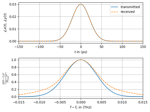
As shown in the previous plot the (isolated) Kerr nonlinearity does not affect the absolute value of the signal’s amplitude but only shifts the phase (see below).
Further, the bandwidth of the transmit signal was slightly increased.
Hint: Increasing the peak power \(p_0\) of the transmitted impuls increases the impact of the Kerr nonlinearity.
[17]:
fig, (ax1) = plt.subplots(1, 1, tight_layout=True)

ax1.plot(t.numpy().flatten(), np.angle(x.numpy().flatten()), '-')
ax1.plot(t.numpy().flatten(), np.angle(y.numpy().flatten()), '--')
ax1.set_xlim(-750, 750)
ax1.set_xlabel("$t$ in (ps)")
ax1.set_ylabel("$\u2220 x(t), \u2220 y(t)$")
ax1.grid()

ax1.legend(['transmitted', 'received'])
plt.tight_layout()

plt.show()
Split-Step Fourier Method
Last, we perform the true SSFM to simulate the impairments (ASE noise, CD, and Kerr nonlinearity) jointly. As this is computationally complex, we compile the channel model before its execution by adding the tf.function decorator.
Channel Configuration
Keeping the former configuration, we only have to increase the number of SSFM simulation steps.
[18]:
n_ssfm = 160 # number of SSFM simulation steps
[19]:
span_ssfm = sionna.channel.optical.SSFM(
            alpha=alpha,
            beta_2=beta_2,
            gamma=gamma,
            f_c=f_c,
            length=length_sp,
            sample_duration=dt,
            n_ssfm=n_ssfm,
            with_amplification=False,
            with_attenuation=True,
            with_dispersion=True,
            with_nonlinearity=True,
            dtype=dtype,
            t_norm=t_norm)

amplifier_ssfm = sionna.channel.optical.EDFA(
            g=g_edfa,
            f=0,
            f_c=f_c,
            dt=dt * t_norm,
            dtype=dtype)

@tf.function
def lumped_amplification_channel_ssfm(inputs):
    (u_0) = inputs

    u = u_0
    for _ in range(1):
        u = span_ssfm(u)
        u = amplifier_ssfm(u)

    return u
Transmission
We transmit the Gaussian impulse over the optical fiber. However, we have now enabled ASE noise, CD, and Kerr nonlinearity.
[20]:
x = g_0
y = lumped_amplification_channel_ssfm(x)

X = tf.signal.fftshift(
    tf.abs(
        tf.cast(dt, dtype) *
        tf.signal.fft(x) /
        tf.cast(tf.math.sqrt(2 * np.pi), dtype)
    ) ** 2
)

Y = tf.signal.fftshift(
    tf.abs(
        tf.cast(dt, dtype) *
        tf.signal.fft(y) /
        tf.cast(tf.math.sqrt(2 * np.pi), dtype)
    ) ** 2
)

X_angle = tf.math.angle(tf.signal.fftshift(tf.signal.fft(x)))
Y_angle = tf.math.angle(tf.signal.fftshift(tf.signal.fft(y)))
[21]:
fig, (ax1, ax2) = plt.subplots(2, 1)

ax1.plot(t.numpy().flatten(), np.abs(x.numpy().flatten())**2, '-')
ax1.plot(t.numpy().flatten(), np.abs(y.numpy().flatten())**2, '--')
ax1.set_xlim(-150, 150)
ax1.set_xlabel(r"$t$ in (ps)")
ax1.set_ylabel(r"$|g(t)|^2$ in (W)")
ax1.grid()

ax2.plot(
    f.numpy().flatten(),
    (X.numpy().flatten()/np.max(X.numpy().flatten())),
    '-')
ax2.plot(
    f.numpy().flatten(),
    (Y.numpy().flatten()/np.max(Y.numpy().flatten())),
    '--')
ax2.set_xlim(-0.015, 0.015)
ax2.set_xlabel(r"$f-f_c$ in (THz)")
ax2.set_ylabel(r"$\frac{|G(f-f_c)|^2}{|G_\mathrm{max}|^2}$")
ax2.grid()

ax1.legend(['transmitted', 'received'])
plt.tight_layout()

plt.show()
[22]:
fig, (ax1) = plt.subplots(1, 1, tight_layout=True)

ax1.plot(t.numpy().flatten(), np.angle(x.numpy().flatten()), '-')
ax1.plot(t.numpy().flatten(), np.angle(y.numpy().flatten()), '--')
ax1.set_xlim(-500, 500)
ax1.set_xlabel("$t$ in (ps)")
ax1.set_ylabel("$\u2220 x(t), \u2220 y(t)$")
ax1.grid()

ax1.legend(['transmitted', 'received'])
plt.tight_layout()

plt.show()
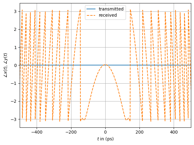
The most interesting observation that one can make here is that the spectrum of the received signal is compressed. This is in contrast to the expected Kerr nonlinearity-induced spectral broadening, and shows that joint application of the fiber effects may result in completely different observations compared to the isolated investigation.
What we can see here, however, is that the Gaussian input impulse is transformed to a higher-order Soliton during propagation. Those require a joint CD and Kerr nonlinearity to exist.
References
[1] René-Jean Essiambre, Gerhard Kramer, Peter J. Winzer, Gerard J. Foschini, and Bernhard Goebel. „Capacity Limits of Optical Fiber Networks“. Journal of Lightwave Technology 28, Nr. 4, pp 662–701, February 2010.