Weighted Belief Propagation Decoding
This notebooks implements the Weighted Belief Propagation (BP) algorithm as proposed by Nachmani et al. in [1]. The main idea is to leverage BP decoding by additional trainable weights that scale each outgoing variable node (VN) and check node (CN) message. These weights provide additional degrees of freedom and can be trained by stochastic gradient descent (SGD) to improve the BP performance for the given code. If all weights are initialized with 1, the algorithm equals the classical BP algorithm and, thus, the concept can be seen as a generalized BP decoder.
Our main focus is to show how Sionna can lower the barrier-to-entry for state-of-the-art research. For this, you will investigate:
How to implement the multi-loss BP decoding with Sionna
How a single scaling factor can lead to similar results
What happens for training of the 5G LDPC code
The setup includes the following components:
LDPC BP Decoder
Gaussian LLR source
Please note that we implement a simplified version of the original algorithm consisting of two major simplifications:
) Only outgoing variable node (VN) messages are weighted. This is possible as the VN operation is linear and it would only increase the memory complexity without increasing the expressive power of the neural network.
) We use the same shared weights for all iterations. This can potentially influence the final performance, however, simplifies the implementation and allows to run the decoder with different number of iterations.
Note: If you are not familiar with all-zero codeword-based simulations please have a look into the Bit-Interleaved Coded Modulation example notebook first.
Table of Contents

GPU Configuration and Imports
[1]:
import os
if os.getenv("CUDA_VISIBLE_DEVICES") is None:
    gpu_num = 0 # Use "" to use the CPU
    os.environ["CUDA_VISIBLE_DEVICES"] = f"{gpu_num}"
os.environ['TF_CPP_MIN_LOG_LEVEL'] = '3'

# Import Sionna
try:
    import sionna
except ImportError as e:
    # Install Sionna if package is not already installed
    import os
    os.system("pip install sionna")
    import sionna

import tensorflow as tf
# Configure the notebook to use only a single GPU and allocate only as much memory as needed
# For more details, see https://www.tensorflow.org/guide/gpu
gpus = tf.config.list_physical_devices('GPU')
if gpus:
    try:
        tf.config.experimental.set_memory_growth(gpus[0], True)
    except RuntimeError as e:
        print(e)
# Avoid warnings from TensorFlow
tf.get_logger().setLevel('ERROR')

# Import required Sionna components
from sionna.fec.ldpc import LDPCBPDecoder, LDPC5GEncoder, LDPC5GDecoder
from sionna.utils.metrics import BitwiseMutualInformation
from sionna.fec.utils import GaussianPriorSource, load_parity_check_examples
from sionna.utils import ebnodb2no, hard_decisions
from sionna.utils.metrics import compute_ber
from sionna.utils.plotting import PlotBER
from tensorflow.keras.losses import BinaryCrossentropy

sionna.config.seed = 42 # Set seed for reproducible random number generation

%matplotlib inline
import matplotlib.pyplot as plt
import numpy as np
Weighted BP for BCH Codes
First, we define the trainable model consisting of:
LDPC BP decoder
Gaussian LLR source
The idea of the multi-loss function in [1] is to average the loss overall iterations, i.e., not just the final estimate is evaluated. This requires to call the BP decoder iteration-wise by setting num_iter=1 and stateful=True such that the decoder will perform a single iteration and returns its current estimate while also providing the internal messages for the next iteration.
A few comments:
We assume the transmission of the all-zero codeword. This allows to train and analyze the decoder without the need of an encoder. Remark: The final decoder can be used for arbitrary codewords.
We directly generate the channel LLRs with
GaussianPriorSource. The equivalent LLR distribution could be achieved by transmitting the all-zero codeword over an AWGN channel with BPSK modulation.For the proposed multi-loss [1] (i.e., the loss is averaged over all iterations), we need to access the decoders intermediate output after each iteration. This is done by calling the decoding function multiple times while setting
statefulto True, i.e., the decoder continuous the decoding process at the last message state.
[2]:
class WeightedBP(tf.keras.Model):
    """System model for BER simulations of weighted BP decoding.

    This model uses `GaussianPriorSource` to mimic the LLRs after demapping of
    QPSK symbols transmitted over an AWGN channel.

    Parameters
    ----------
        pcm: ndarray
            The parity-check matrix of the code under investigation.

        num_iter: int
            Number of BP decoding iterations.


    Input
    -----
        batch_size: int or tf.int
            The batch_size used for the simulation.

        ebno_db: float or tf.float
            A float defining the simulation SNR.

    Output
    ------
        (u, u_hat, loss):
            Tuple:

        u: tf.float32
            A tensor of shape `[batch_size, k] of 0s and 1s containing the transmitted information bits.

        u_hat: tf.float32
            A tensor of shape `[batch_size, k] of 0s and 1s containing the estimated information bits.

        loss: tf.float32
            Binary cross-entropy loss between `u` and `u_hat`.
    """
    def __init__(self, pcm, num_iter=5):
        super().__init__()

        # init components
        self.decoder = LDPCBPDecoder(pcm,
                                     num_iter=1, # iterations are done via outer loop (to access intermediate results for multi-loss)
                                     stateful=True, # decoder stores internal messages after call
                                     hard_out=False, # we need to access soft-information
                                     cn_type="boxplus",
                                     trainable=True) # the decoder must be trainable, otherwise no weights are generated

        # used to generate llrs during training (see example notebook on all-zero codeword trick)
        self.llr_source = GaussianPriorSource()
        self._num_iter = num_iter

        self._bce = BinaryCrossentropy(from_logits=True)

    def call(self, batch_size, ebno_db):
        noise_var = ebnodb2no(ebno_db,
                              num_bits_per_symbol=2, # QPSK
                              coderate=coderate)

        # all-zero CW to calculate loss / BER
        c = tf.zeros([batch_size, n])

        # Gaussian LLR source
        llr = self.llr_source([[batch_size, n], noise_var])

        # --- implement multi-loss as proposed by Nachmani et al. [1]---
        loss = 0
        msg_vn = None # internal state of decoder
        for i in range(self._num_iter):
            c_hat, msg_vn = self.decoder((llr, msg_vn)) # perform one decoding iteration; decoder returns soft-values
            loss += self._bce(c, c_hat)  # add loss after each iteration

        loss /= self._num_iter # scale loss by number of iterations

        return c, c_hat, loss
Load a parity-check matrix used for the experiment. We use the same BCH(63,45) code as in [1]. The code can be replaced by any parity-check matrix of your choice.
[3]:
pcm_id = 1 # (63,45) BCH code parity check matrix
pcm, k , n, coderate = load_parity_check_examples(pcm_id=pcm_id, verbose=True)

num_iter = 10 # set number of decoding iterations

# and initialize the model
model = WeightedBP(pcm=pcm, num_iter=num_iter)
n: 63, k: 45, coderate: 0.714
Note: weighted BP tends to work better for small number of iterations. The effective gains (compared to the baseline with same number of iterations) vanish with more iterations.
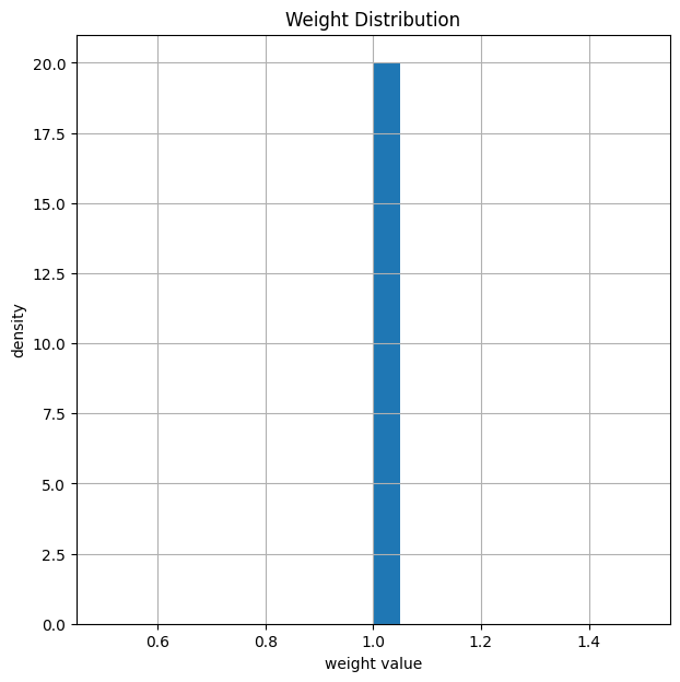
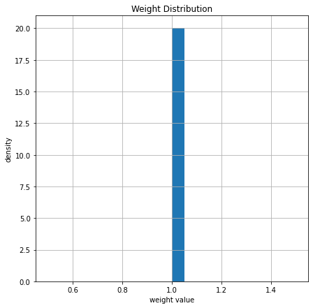
Weights before Training and Simulation of BER
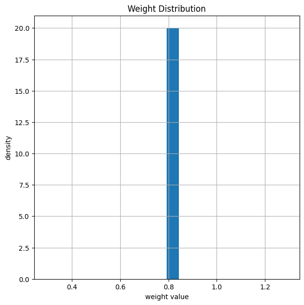
Let us plot the weights after initialization of the decoder to verify that everything is properly initialized. This is equivalent the classical BP decoder.
[4]:
# count number of weights/edges
print("Total number of weights: ", np.size(model.decoder.get_weights()))

# and show the weight distribution
model.decoder.show_weights()
Total number of weights: 432
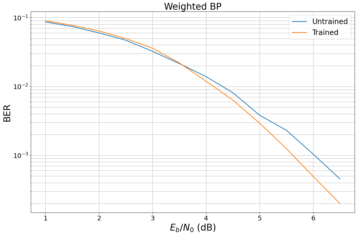
We first simulate (and store) the BER performance before training. For this, we use the PlotBER class, which provides a convenient way to store the results for later comparison.
[5]:
# SNR to simulate the results
ebno_dbs = np.array(np.arange(1, 7, 0.5))
mc_iters = 100 # number of Monte Carlo iterations

# we generate a new PlotBER() object to simulate, store and plot the BER results
ber_plot = PlotBER("Weighted BP")

# simulate and plot the BER curve of the untrained decoder
ber_plot.simulate(model,
                  ebno_dbs=ebno_dbs,
                  batch_size=1000,
                  num_target_bit_errors=2000, # stop sim after 2000 bit errors
                  legend="Untrained",
                  soft_estimates=True,
                  max_mc_iter=mc_iters,
                  forward_keyboard_interrupt=False);
EbNo [dB] |        BER |       BLER |  bit errors |    num bits | block errors |  num blocks | runtime [s] |    status
---------------------------------------------------------------------------------------------------------------------------------------
      1.0 | 8.6508e-02 | 9.6500e-01 |        5450 |       63000 |          965 |        1000 |         2.8 |reached target bit errors
      1.5 | 7.4175e-02 | 9.2100e-01 |        4673 |       63000 |          921 |        1000 |         0.3 |reached target bit errors
      2.0 | 5.9952e-02 | 8.0400e-01 |        3777 |       63000 |          804 |        1000 |         0.3 |reached target bit errors
      2.5 | 4.6921e-02 | 6.8300e-01 |        2956 |       63000 |          683 |        1000 |         0.3 |reached target bit errors
      3.0 | 3.2381e-02 | 4.8800e-01 |        2040 |       63000 |          488 |        1000 |         0.3 |reached target bit errors
      3.5 | 2.1516e-02 | 3.5450e-01 |        2711 |      126000 |          709 |        2000 |         0.6 |reached target bit errors
      4.0 | 1.3878e-02 | 2.4100e-01 |        2623 |      189000 |          723 |        3000 |         0.9 |reached target bit errors
      4.5 | 8.1230e-03 | 1.4550e-01 |        2047 |      252000 |          582 |        4000 |         1.2 |reached target bit errors
      5.0 | 3.8272e-03 | 7.3111e-02 |        2170 |      567000 |          658 |        9000 |         2.6 |reached target bit errors
      5.5 | 2.3095e-03 | 4.3857e-02 |        2037 |      882000 |          614 |       14000 |         4.1 |reached target bit errors
      6.0 | 1.0420e-03 | 1.9806e-02 |        2035 |     1953000 |          614 |       31000 |         9.1 |reached target bit errors
      6.5 | 4.5495e-04 | 9.3239e-03 |        2035 |     4473000 |          662 |       71000 |        20.7 |reached target bit errors
Training
We now train the model for a fixed number of SGD training iterations.
Note: this is a very basic implementation of the training loop. You can also try more sophisticated training loops with early stopping, different hyper-parameters or optimizers etc.
[6]:
# training parameters
batch_size = 1000
train_iter = 200
ebno_db = 4.0
clip_value_grad = 10 # gradient clipping for stable training convergence

# bmi is used as metric to evaluate the intermediate results
bmi = BitwiseMutualInformation()

# try also different optimizers or different hyperparameters
optimizer = tf.keras.optimizers.Adam(learning_rate=1e-2)

for it in range(0, train_iter):
    with tf.GradientTape() as tape:
        b, llr, loss = model(batch_size, ebno_db)

    grads = tape.gradient(loss, model.trainable_variables)
    grads = tf.clip_by_value(grads, -clip_value_grad, clip_value_grad, name=None)
    optimizer.apply_gradients(zip(grads, model.trainable_weights))

    # calculate and print intermediate metrics
    # only for information
    # this has no impact on the training
    if it%10==0: # evaluate every 10 iterations
        # calculate ber from received LLRs
        b_hat = hard_decisions(llr) # hard decided LLRs first
        ber = compute_ber(b, b_hat)
        # and print results
        mi = bmi(b, llr).numpy() # calculate bit-wise mutual information
        l = loss.numpy() # copy loss to numpy for printing
        print(f"Current loss: {l:3f} ber: {ber:.4f} bmi: {mi:.3f}".format())
        bmi.reset_states() # reset the BMI metric
WARNING: All log messages before absl::InitializeLog() is called are written to STDERR
I0000 00:00:1727421292.987160  408205 device_compiler.h:186] Compiled cluster using XLA!  This line is logged at most once for the lifetime of the process.
Current loss: 0.050724 ber: 0.0126 bmi: 0.932
Current loss: 0.053875 ber: 0.0131 bmi: 0.943
Current loss: 0.053504 ber: 0.0135 bmi: 0.931
Current loss: 0.049400 ber: 0.0126 bmi: 0.931
Current loss: 0.062802 ber: 0.0129 bmi: 0.902
Current loss: 0.045709 ber: 0.0121 bmi: 0.945
Current loss: 0.037912 ber: 0.0111 bmi: 0.957
Current loss: 0.049750 ber: 0.0134 bmi: 0.930
Current loss: 0.040948 ber: 0.0123 bmi: 0.946
Current loss: 0.039643 ber: 0.0110 bmi: 0.948
Current loss: 0.041965 ber: 0.0120 bmi: 0.947
Current loss: 0.038897 ber: 0.0117 bmi: 0.946
Current loss: 0.044827 ber: 0.0128 bmi: 0.937
Current loss: 0.048558 ber: 0.0135 bmi: 0.936
Current loss: 0.040099 ber: 0.0132 bmi: 0.949
Current loss: 0.044894 ber: 0.0136 bmi: 0.936
Current loss: 0.039783 ber: 0.0122 bmi: 0.951
Current loss: 0.038629 ber: 0.0119 bmi: 0.952
Current loss: 0.045271 ber: 0.0146 bmi: 0.937
Current loss: 0.037925 ber: 0.0114 bmi: 0.954
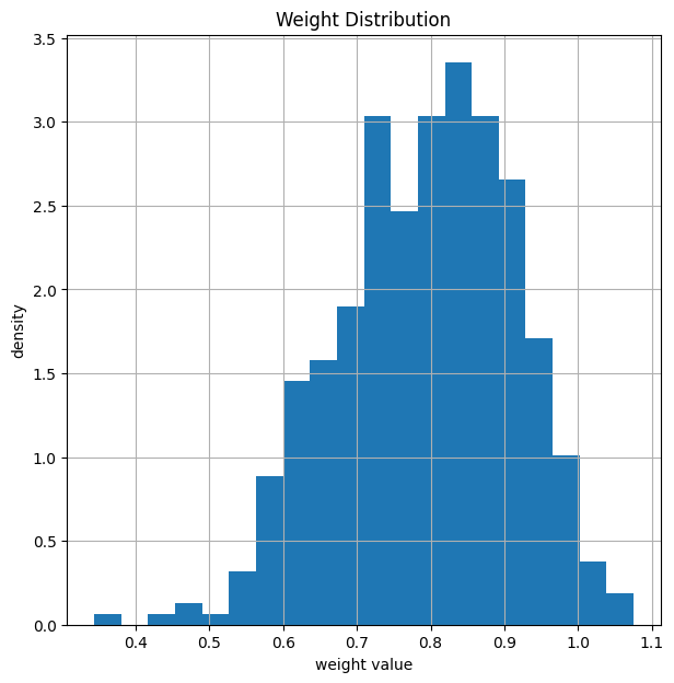
Results
After training, the weights of the decoder have changed. In average, the weights are smaller after training.
[7]:
model.decoder.show_weights() # show weights AFTER training
And let us compare the new BER performance. For this, we can simply call the ber_plot.simulate() function again as it internally stores all previous results (if add_results is True).
[8]:
ebno_dbs = np.array(np.arange(1, 7, 0.5))
batch_size = 10000
mc_ites = 100

ber_plot.simulate(model,
                  ebno_dbs=ebno_dbs,
                  batch_size=1000,
                  num_target_bit_errors=2000, # stop sim after 2000 bit errors
                  legend="Trained",
                  max_mc_iter=mc_iters,
                  soft_estimates=True);
EbNo [dB] |        BER |       BLER |  bit errors |    num bits | block errors |  num blocks | runtime [s] |    status
---------------------------------------------------------------------------------------------------------------------------------------
      1.0 | 9.0000e-02 | 9.9400e-01 |        5670 |       63000 |          994 |        1000 |         0.3 |reached target bit errors
      1.5 | 7.7349e-02 | 9.7500e-01 |        4873 |       63000 |          975 |        1000 |         0.3 |reached target bit errors
      2.0 | 6.3905e-02 | 9.3500e-01 |        4026 |       63000 |          935 |        1000 |         0.3 |reached target bit errors
      2.5 | 4.9587e-02 | 8.1400e-01 |        3124 |       63000 |          814 |        1000 |         0.3 |reached target bit errors
      3.0 | 3.5905e-02 | 6.3300e-01 |        2262 |       63000 |          633 |        1000 |         0.3 |reached target bit errors
      3.5 | 2.1984e-02 | 4.1200e-01 |        2770 |      126000 |          824 |        2000 |         0.6 |reached target bit errors
      4.0 | 1.1884e-02 | 2.3600e-01 |        2246 |      189000 |          708 |        3000 |         0.9 |reached target bit errors
      4.5 | 6.3492e-03 | 1.2850e-01 |        2400 |      378000 |          771 |        6000 |         1.7 |reached target bit errors
      5.0 | 2.9293e-03 | 6.1909e-02 |        2030 |      693000 |          681 |       11000 |         3.2 |reached target bit errors
      5.5 | 1.2521e-03 | 2.9385e-02 |        2051 |     1638000 |          764 |       26000 |         7.5 |reached target bit errors
      6.0 | 4.9353e-04 | 1.2431e-02 |        2021 |     4095000 |          808 |       65000 |        18.6 |reached target bit errors
      6.5 | 1.9921e-04 | 5.6500e-03 |        1255 |     6300000 |          565 |      100000 |        28.9 |reached max iter
Further Experiments
You will now see that the memory footprint can be drastically reduced by using the same weight for all messages. In the second part we will apply the concept to the 5G LDPC codes.
Damped BP
It is well-known that scaling of LLRs / messages can help to improve the performance of BP decoding in some scenarios [3,4]. In particular, this works well for very short codes such as the code we are currently analyzing.
We now follow the basic idea of [2] and scale all weights with the same scalar.
[9]:
# get weights of trained model
weights_bp = model.decoder.get_weights()

# calc mean value of weights
damping_factor = tf.reduce_mean(weights_bp)

# set all weights to the SAME constant scaling
weights_damped = tf.ones_like(weights_bp) * damping_factor

# and apply the new weights
model.decoder.set_weights(weights_damped)

# let us have look at the new weights again
model.decoder.show_weights()

# and simulate the BER again
leg_str = f"Damped BP (scaling factor {damping_factor.numpy():.3f})"
ber_plot.simulate(model,
                  ebno_dbs=ebno_dbs,
                  batch_size=1000,
                  num_target_bit_errors=2000, # stop sim after 2000 bit errors
                  legend=leg_str,
                  max_mc_iter=mc_iters,
                  soft_estimates=True);
EbNo [dB] |        BER |       BLER |  bit errors |    num bits | block errors |  num blocks | runtime [s] |    status
---------------------------------------------------------------------------------------------------------------------------------------
      1.0 | 8.8667e-02 | 9.9600e-01 |        5586 |       63000 |          996 |        1000 |         0.3 |reached target bit errors
      1.5 | 7.5619e-02 | 9.7700e-01 |        4764 |       63000 |          977 |        1000 |         0.3 |reached target bit errors
      2.0 | 6.3381e-02 | 9.1500e-01 |        3993 |       63000 |          915 |        1000 |         0.3 |reached target bit errors
      2.5 | 4.9016e-02 | 8.0700e-01 |        3088 |       63000 |          807 |        1000 |         0.3 |reached target bit errors
      3.0 | 3.3476e-02 | 5.9500e-01 |        2109 |       63000 |          595 |        1000 |         0.3 |reached target bit errors
      3.5 | 2.1222e-02 | 3.9400e-01 |        2674 |      126000 |          788 |        2000 |         0.6 |reached target bit errors
      4.0 | 1.2651e-02 | 2.4033e-01 |        2391 |      189000 |          721 |        3000 |         0.8 |reached target bit errors
      4.5 | 5.9339e-03 | 1.1867e-01 |        2243 |      378000 |          712 |        6000 |         1.7 |reached target bit errors
      5.0 | 2.7910e-03 | 5.7917e-02 |        2110 |      756000 |          695 |       12000 |         3.4 |reached target bit errors
      5.5 | 1.2952e-03 | 2.9120e-02 |        2040 |     1575000 |          728 |       25000 |         7.0 |reached target bit errors
      6.0 | 5.0920e-04 | 1.2746e-02 |        2021 |     3969000 |          803 |       63000 |        17.5 |reached target bit errors
      6.5 | 2.2841e-04 | 5.6900e-03 |        1439 |     6300000 |          569 |      100000 |        28.8 |reached max iter
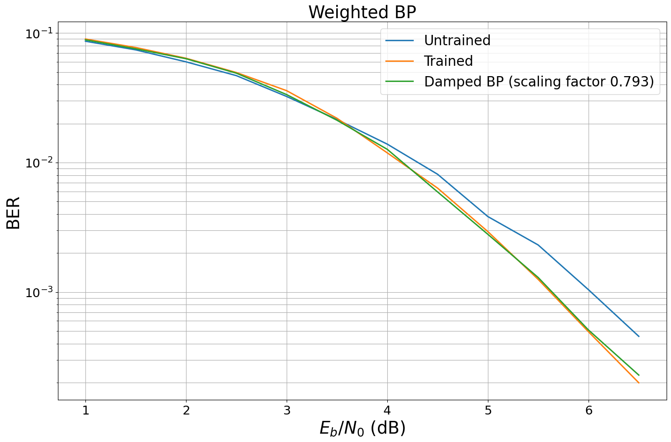
When looking at the results, we observe almost the same performance although we only scale by a single scalar. This implies that the number of weights of our model is by far too large and the memory footprint could be reduced significantly. However, isn’t it fascinating to see that this simple concept of weighted BP leads to the same results as the concept of damped BP?
Note: for more iterations it could be beneficial to implement an individual damping per iteration.
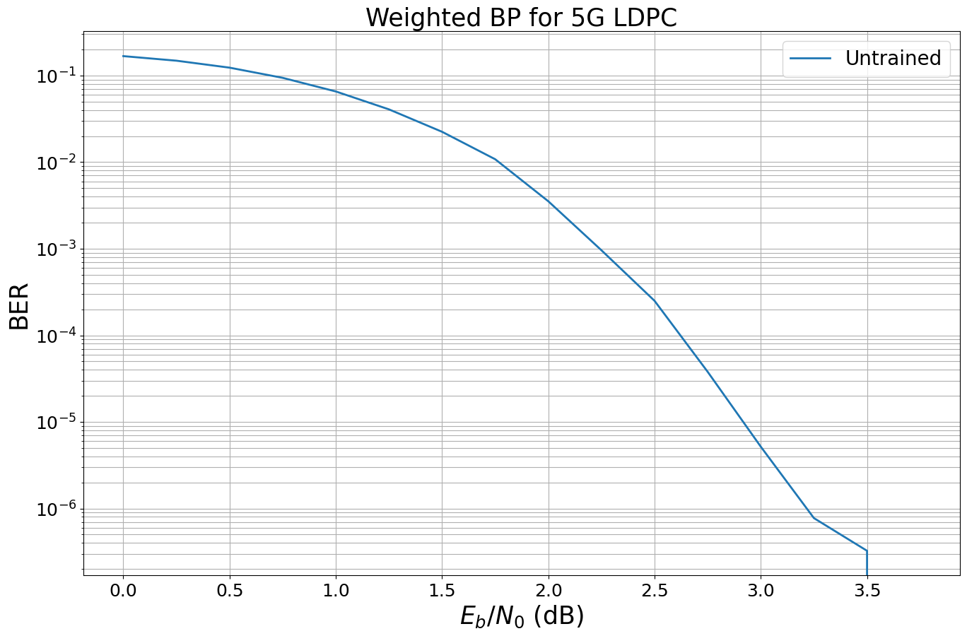
Learning the 5G LDPC Code
In this Section, you will experience what happens if we apply the same concept to the 5G LDPC code (including rate matching).
For this, we need to define a new model.
[10]:
class WeightedBP5G(tf.keras.Model):
    """System model for BER simulations of weighted BP decoding for 5G LDPC codes.

    This model uses `GaussianPriorSource` to mimic the LLRs after demapping of
    QPSK symbols transmitted over an AWGN channel.

    Parameters
    ----------
        k: int
            Number of information bits per codeword.

        n: int
            Codeword length.

        num_iter: int
            Number of BP decoding iterations.

    Input
    -----
        batch_size: int or tf.int
            The batch_size used for the simulation.

        ebno_db: float or tf.float
            A float defining the simulation SNR.

    Output
    ------
        (u, u_hat, loss):
            Tuple:

        u: tf.float32
            A tensor of shape `[batch_size, k] of 0s and 1s containing the transmitted information bits.

        u_hat: tf.float32
            A tensor of shape `[batch_size, k] of 0s and 1s containing the estimated information bits.

        loss: tf.float32
            Binary cross-entropy loss between `u` and `u_hat`.
    """
    def __init__(self, k, n, num_iter=20):
        super().__init__()

        # we need to initialize an encoder for the 5G parameters
        self.encoder = LDPC5GEncoder(k, n)
        self.decoder = LDPC5GDecoder(self.encoder,
                                     num_iter=1, # iterations are done via outer loop (to access intermediate results for multi-loss)
                                     stateful=True,
                                     hard_out=False,
                                     cn_type="boxplus",
                                     trainable=True)

        self.llr_source = GaussianPriorSource()
        self._num_iter = num_iter
        self._coderate = k/n

        self._bce = BinaryCrossentropy(from_logits=True)
    def call(self, batch_size, ebno_db):

        noise_var = ebnodb2no(ebno_db,
                              num_bits_per_symbol=2, # QPSK
                              coderate=self._coderate)

        # BPSK modulated all-zero CW
        c = tf.zeros([batch_size, k]) # decoder only returns info bits

        # use fake llrs from GA
        # works as BP is symmetric
        llr = self.llr_source([[batch_size, n], noise_var])

        # --- implement multi-loss is proposed by Nachmani et al. ---
        loss = 0
        msg_vn = None
        for i in range(self._num_iter):
            c_hat, msg_vn = self.decoder((llr, msg_vn)) # perform one decoding iteration; decoder returns soft-values
            loss += self._bce(c, c_hat)  # add loss after each iteration

        return c, c_hat, loss
[11]:
# generate model
num_iter = 10
k = 400
n = 800

model5G = WeightedBP5G(k, n, num_iter=num_iter)

# generate baseline BER
ebno_dbs = np.array(np.arange(0, 4, 0.25))
mc_iters = 100 # number of monte carlo iterations
ber_plot_5G = PlotBER("Weighted BP for 5G LDPC")

# simulate the untrained performance
ber_plot_5G.simulate(model5G,
                     ebno_dbs=ebno_dbs,
                     batch_size=1000,
                     num_target_bit_errors=2000, # stop sim after 2000 bit errors
                     legend="Untrained",
                     soft_estimates=True,
                     max_mc_iter=mc_iters);
EbNo [dB] |        BER |       BLER |  bit errors |    num bits | block errors |  num blocks | runtime [s] |    status
---------------------------------------------------------------------------------------------------------------------------------------
      0.0 | 1.6760e-01 | 1.0000e+00 |       67039 |      400000 |         1000 |        1000 |         0.4 |reached target bit errors
     0.25 | 1.4844e-01 | 1.0000e+00 |       59374 |      400000 |         1000 |        1000 |         0.4 |reached target bit errors
      0.5 | 1.2333e-01 | 9.9700e-01 |       49331 |      400000 |          997 |        1000 |         0.4 |reached target bit errors
     0.75 | 9.4090e-02 | 9.8500e-01 |       37636 |      400000 |          985 |        1000 |         0.4 |reached target bit errors
      1.0 | 6.5505e-02 | 9.2400e-01 |       26202 |      400000 |          924 |        1000 |         0.4 |reached target bit errors
     1.25 | 4.0692e-02 | 8.1500e-01 |       16277 |      400000 |          815 |        1000 |         0.4 |reached target bit errors
      1.5 | 2.2415e-02 | 6.2200e-01 |        8966 |      400000 |          622 |        1000 |         0.4 |reached target bit errors
     1.75 | 1.0802e-02 | 3.8600e-01 |        4321 |      400000 |          386 |        1000 |         0.4 |reached target bit errors
      2.0 | 3.5325e-03 | 1.9200e-01 |        2826 |      800000 |          384 |        2000 |         0.8 |reached target bit errors
     2.25 | 9.6042e-04 | 7.7167e-02 |        2305 |     2400000 |          463 |        6000 |         2.3 |reached target bit errors
      2.5 | 2.5036e-04 | 2.3667e-02 |        2103 |     8400000 |          497 |       21000 |         8.2 |reached target bit errors
     2.75 | 3.7900e-05 | 4.9500e-03 |        1516 |    40000000 |          495 |      100000 |        38.6 |reached max iter
      3.0 | 5.1750e-06 | 1.0000e-03 |         207 |    40000000 |          100 |      100000 |        38.7 |reached max iter
     3.25 | 7.7500e-07 | 1.6000e-04 |          31 |    40000000 |           16 |      100000 |        38.7 |reached max iter
      3.5 | 3.2500e-07 | 4.0000e-05 |          13 |    40000000 |            4 |      100000 |        39.2 |reached max iter
     3.75 | 0.0000e+00 | 0.0000e+00 |           0 |    40000000 |            0 |      100000 |        39.0 |reached max iter

Simulation stopped as no error occurred @ EbNo = 3.8 dB.
And let’s train this new model.
[12]:
# training parameters
batch_size = 1000
train_iter = 200
clip_value_grad = 10 # gradient clipping seems to be important

# smaller training SNR as the new code is longer (=stronger) than before
ebno_db = 1.5 # rule of thumb: train at ber = 1e-2

# only used as metric
bmi = BitwiseMutualInformation()

# try also different optimizers or different hyperparameters
optimizer = tf.keras.optimizers.Adam(learning_rate=1e-2)

# and let's go
for it in range(0, train_iter):
    with tf.GradientTape() as tape:
        b, llr, loss = model5G(batch_size, ebno_db)

    grads = tape.gradient(loss, model5G.trainable_variables)
    grads = tf.clip_by_value(grads, -clip_value_grad, clip_value_grad, name=None)
    optimizer.apply_gradients(zip(grads, model5G.trainable_weights))

    # calculate and print intermediate metrics
    if it%10==0:
        # calculate ber
        b_hat = hard_decisions(llr)
        ber = compute_ber(b, b_hat)
        # and print results
        mi = bmi(b, llr).numpy()
        l = loss.numpy()
        print(f"Current loss: {l:3f} ber: {ber:.4f} bmi: {mi:.3f}".format())
        bmi.reset_states()
Current loss: 1.728374 ber: 0.0227 bmi: 0.917
Current loss: 1.686895 ber: 0.0210 bmi: 0.924
Current loss: 1.701802 ber: 0.0199 bmi: 0.926
Current loss: 1.723080 ber: 0.0214 bmi: 0.922
Current loss: 1.757810 ber: 0.0236 bmi: 0.913
Current loss: 1.689232 ber: 0.0200 bmi: 0.926
Current loss: 1.731120 ber: 0.0219 bmi: 0.918
Current loss: 1.683933 ber: 0.0197 bmi: 0.928
Current loss: 1.732217 ber: 0.0219 bmi: 0.918
Current loss: 1.705418 ber: 0.0218 bmi: 0.920
Current loss: 1.726237 ber: 0.0218 bmi: 0.920
Current loss: 1.721895 ber: 0.0219 bmi: 0.919
Current loss: 1.713015 ber: 0.0211 bmi: 0.922
Current loss: 1.732242 ber: 0.0225 bmi: 0.917
Current loss: 1.696066 ber: 0.0201 bmi: 0.926
Current loss: 1.678042 ber: 0.0191 bmi: 0.929
Current loss: 1.711135 ber: 0.0205 bmi: 0.925
Current loss: 1.712982 ber: 0.0209 bmi: 0.924
Current loss: 1.708192 ber: 0.0209 bmi: 0.923
Current loss: 1.704635 ber: 0.0206 bmi: 0.923
We now simulate the new results and compare it to the untrained results.
[13]:
ebno_dbs = np.array(np.arange(0, 4, 0.25))
batch_size = 1000
mc_iters = 100

ber_plot_5G.simulate(model5G,
                     ebno_dbs=ebno_dbs,
                     batch_size=batch_size,
                     num_target_bit_errors=2000, # stop sim after 2000 bit errors
                     legend="Trained",
                     max_mc_iter=mc_iters,
                     soft_estimates=True);
EbNo [dB] |        BER |       BLER |  bit errors |    num bits | block errors |  num blocks | runtime [s] |    status
---------------------------------------------------------------------------------------------------------------------------------------
      0.0 | 1.6626e-01 | 1.0000e+00 |       66505 |      400000 |         1000 |        1000 |         0.4 |reached target bit errors
     0.25 | 1.4691e-01 | 1.0000e+00 |       58764 |      400000 |         1000 |        1000 |         0.4 |reached target bit errors
      0.5 | 1.2461e-01 | 9.9900e-01 |       49845 |      400000 |          999 |        1000 |         0.4 |reached target bit errors
     0.75 | 9.7850e-02 | 9.9300e-01 |       39140 |      400000 |          993 |        1000 |         0.4 |reached target bit errors
      1.0 | 6.7318e-02 | 9.3500e-01 |       26927 |      400000 |          935 |        1000 |         0.4 |reached target bit errors
     1.25 | 4.3007e-02 | 8.3100e-01 |       17203 |      400000 |          831 |        1000 |         0.4 |reached target bit errors
      1.5 | 2.1902e-02 | 6.2100e-01 |        8761 |      400000 |          621 |        1000 |         0.4 |reached target bit errors
     1.75 | 8.6150e-03 | 3.6600e-01 |        3446 |      400000 |          366 |        1000 |         0.4 |reached target bit errors
      2.0 | 2.5388e-03 | 1.6500e-01 |        2031 |      800000 |          330 |        2000 |         0.8 |reached target bit errors
     2.25 | 8.6375e-04 | 6.2833e-02 |        2073 |     2400000 |          377 |        6000 |         2.3 |reached target bit errors
      2.5 | 1.8464e-04 | 1.9036e-02 |        2068 |    11200000 |          533 |       28000 |        10.9 |reached target bit errors
     2.75 | 3.3400e-05 | 4.5200e-03 |        1336 |    40000000 |          452 |      100000 |        38.8 |reached max iter
      3.0 | 4.4000e-06 | 8.4000e-04 |         176 |    40000000 |           84 |      100000 |        38.6 |reached max iter
     3.25 | 6.2500e-07 | 1.7000e-04 |          25 |    40000000 |           17 |      100000 |        38.7 |reached max iter
      3.5 | 5.0000e-08 | 2.0000e-05 |           2 |    40000000 |            2 |      100000 |        38.5 |reached max iter
     3.75 | 0.0000e+00 | 0.0000e+00 |           0 |    40000000 |            0 |      100000 |        38.5 |reached max iter

Simulation stopped as no error occurred @ EbNo = 3.8 dB.
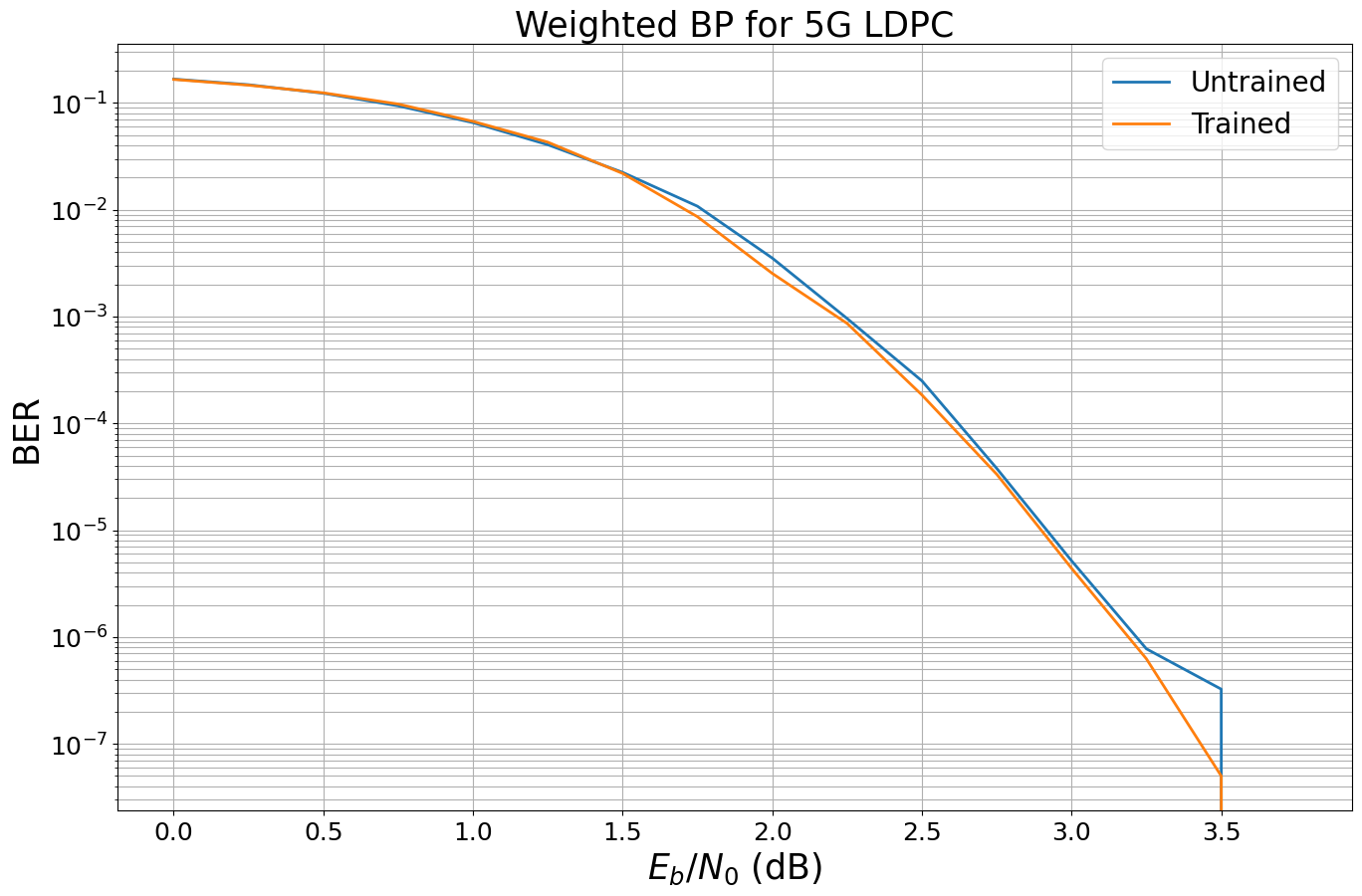
Unfortunately, we observe only very minor gains for the 5G LDPC code. We empirically observed that gain vanishes for more iterations and longer codewords, i.e., for most practical use-cases of the 5G LDPC code the gains are only minor.
However, there may be other codes on graphs that benefit from the principle idea of weighted BP - or other channel setups? Feel free to adjust this notebook and train for your favorite code / channel.
Other ideas for own experiments:
Implement weighted BP with unique weights per iteration.
Apply the concept to (scaled) min-sum decoding as in [5].
Can you replace the complete CN update by a neural network?
Verify the results from all-zero simulations for a real system simulation with explicit encoder and random data
What happens in combination with higher order modulation?
References
[1] E. Nachmani, Y. Be’ery and D. Burshtein, “Learning to Decode Linear Codes Using Deep Learning,” IEEE Annual Allerton Conference on Communication, Control, and Computing (Allerton), pp. 341-346., 2016. https://arxiv.org/pdf/1607.04793.pdf
[2] M. Lian, C. Häger, and H. Pfister, “What can machine learning teach us about communications?” IEEE Information Theory Workshop (ITW), pp. 1-5. 2018.
[3] ] M. Pretti, “A message passing algorithm with damping,” J. Statist. Mech.: Theory Practice, p. 11008, Nov. 2005.
[4] J.S. Yedidia, W.T. Freeman and Y. Weiss, “Constructing free energy approximations and Generalized Belief Propagation algorithms,” IEEE Transactions on Information Theory, 2005.
[5] E. Nachmani, E. Marciano, L. Lugosch, W. Gross, D. Burshtein and Y. Be’ery, “Deep learning methods for improved decoding of linear codes,” IEEE Journal of Selected Topics in Signal Processing, vol. 12, no. 1, pp.119-131, 2018.