Wireless

This module provides layers and functions that implement wireless channel models. Models currently available include AWGN, flat-fading with (optional) SpatialCorrelation, RayleighBlockFading, as well as models from the 3rd Generation Partnership Project (3GPP) [TR38901]: TDL, CDL, UMi, UMa, and RMa. It is also possible to use externally generated CIRs.

Apart from flat-fading, all of these models generate channel impulse responses (CIRs) that can then be used to implement a channel transfer function in the time domain or assuming an OFDM waveform.

This is achieved using the different functions, classes, and Keras layers which operate as shown in the figures below.

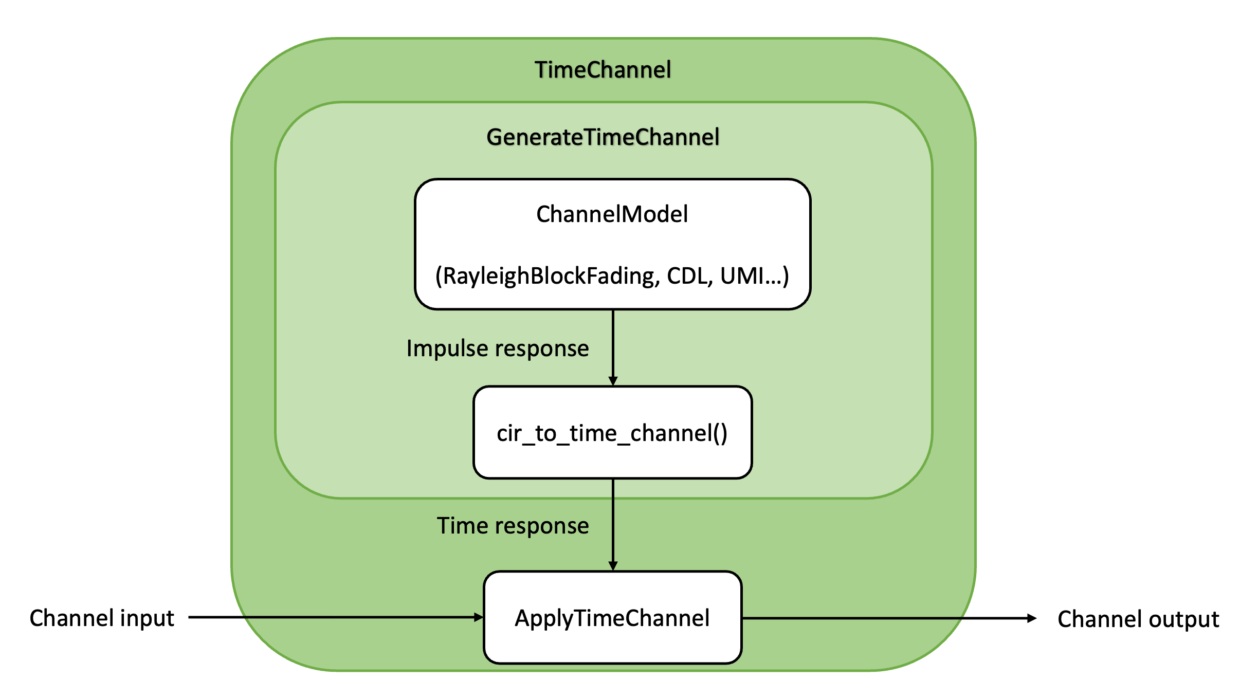
Fig. 7 Channel module architecture for time domain simulations.

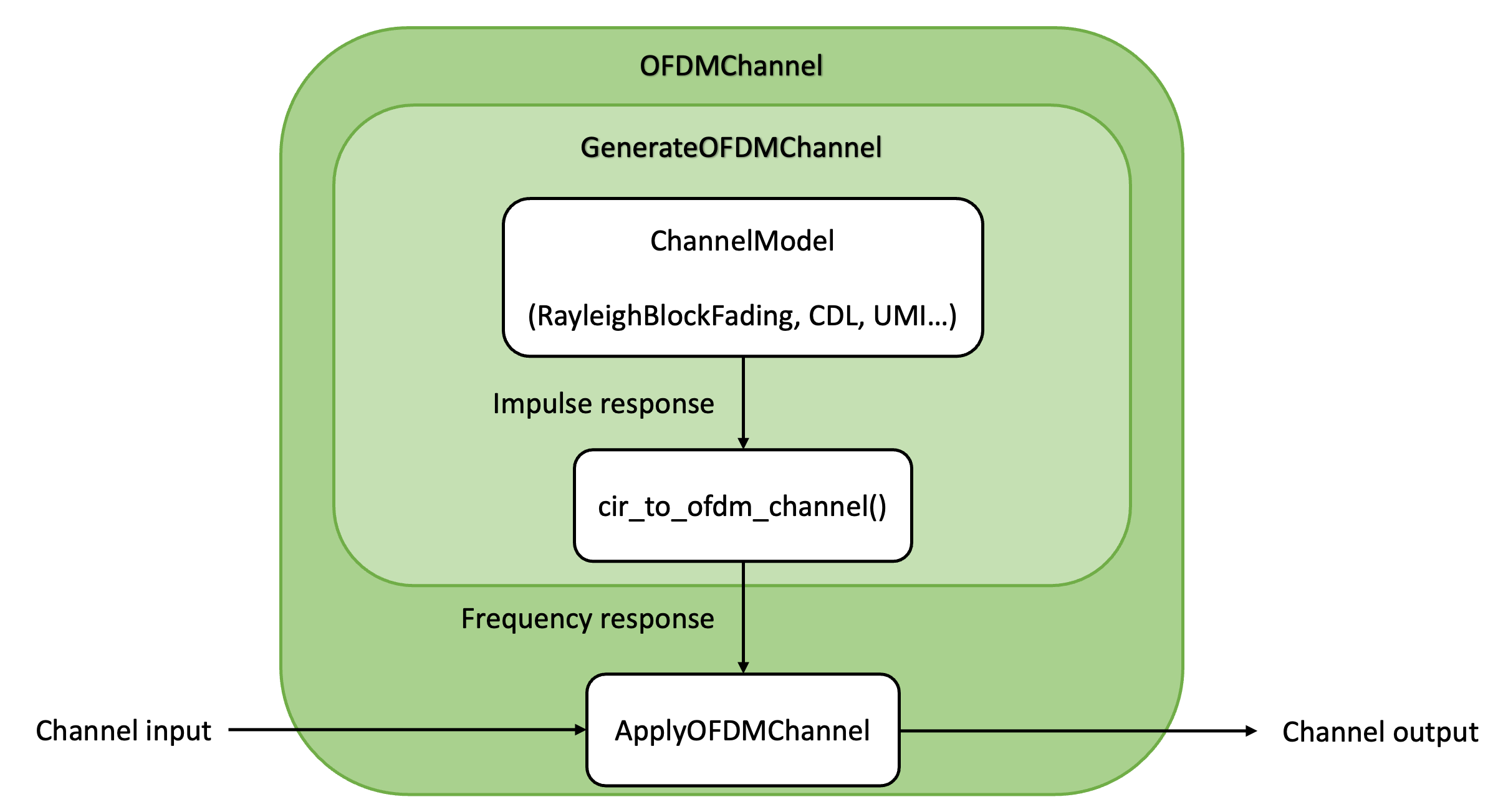
Fig. 8 Channel module architecture for simulations assuming OFDM waveform.

A channel model generate CIRs from which channel responses in the time domain or in the frequency domain are computed using the cir_to_time_channel() or cir_to_ofdm_channel() functions, respectively. If one does not need access to the raw CIRs, the GenerateTimeChannel and GenerateOFDMChannel classes can be used to conveniently sample CIRs and generate channel responses in the desired domain.

Once the channel responses in the time or frequency domain are computed, they can be applied to the channel input using the ApplyTimeChannel or ApplyOFDMChannel Keras layers.

The following code snippets show how to setup and run a Rayleigh block fading model assuming an OFDM waveform, and without accessing the CIRs or channel responses. This is the easiest way to setup a channel model. Setting-up other models is done in a similar way, except for AWGN (see the AWGN class documentation).

rayleigh = RayleighBlockFading(num_rx = 1,
                               num_rx_ant = 32,
                               num_tx = 4,
                               num_tx_ant = 2)

channel  = OFDMChannel(channel_model = rayleigh,
                       resource_grid = rg)

where rg is an instance of ResourceGrid.

Running the channel model is done as follows:

# x is the channel input
# no is the noise variance
y = channel([x, no])

To use the time domain representation of the channel, one can use TimeChannel instead of OFDMChannel.

If access to the channel responses is needed, one can separate their generation from their application to the channel input by setting up the channel model as follows:

rayleigh = RayleighBlockFading(num_rx = 1,
                               num_rx_ant = 32,
                               num_tx = 4,
                               num_tx_ant = 2)

generate_channel = GenerateOFDMChannel(channel_model = rayleigh,
                                       resource_grid = rg)

apply_channel = ApplyOFDMChannel()

where rg is an instance of ResourceGrid. Running the channel model is done as follows:

# Generate a batch of channel responses
h = generate_channel(batch_size)
# Apply the channel
# x is the channel input
# no is the noise variance
y = apply_channel([x, h, no])

Generating and applying the channel in the time domain can be achieved by using GenerateTimeChannel and ApplyTimeChannel instead of GenerateOFDMChannel and ApplyOFDMChannel, respectively.

To access the CIRs, setting up the channel can be done as follows:

rayleigh = RayleighBlockFading(num_rx = 1,
                               num_rx_ant = 32,
                               num_tx = 4,
                               num_tx_ant = 2)

apply_channel = ApplyOFDMChannel()

and running the channel model as follows:

cir = rayleigh(batch_size)
h = cir_to_ofdm_channel(frequencies, *cir)
y = apply_channel([x, h, no])

where frequencies are the subcarrier frequencies in the baseband, which can be computed using the subcarrier_frequencies() utility function.

Applying the channel in the time domain can be done by using cir_to_time_channel() and ApplyTimeChannel instead of cir_to_ofdm_channel() and ApplyOFDMChannel, respectively.

For the purpose of the present document, the following symbols apply:

\(N_T (u)\)	Number of transmitters (transmitter index)
\(N_R (v)\)	Number of receivers (receiver index)
\(N_{TA} (k)\)	Number of antennas per transmitter (transmit antenna index)
\(N_{RA} (l)\)	Number of antennas per receiver (receive antenna index)
\(N_S (s)\)	Number of OFDM symbols (OFDM symbol index)
\(N_F (n)\)	Number of subcarriers (subcarrier index)
\(N_B (b)\)	Number of time samples forming the channel input (baseband symbol index)
\(L_{\text{min}}\)	Smallest time-lag for the discrete complex baseband channel
\(L_{\text{max}}\)	Largest time-lag for the discrete complex baseband channel
\(M (m)\)	Number of paths (clusters) forming a power delay profile (path index)
\(\tau_m(t)\)	\(m^{th}\) path (cluster) delay at time step \(t\)
\(a_m(t)\)	\(m^{th}\) path (cluster) complex coefficient at time step \(t\)
\(\Delta_f\)	Subcarrier spacing
\(W\)	Bandwidth
\(N_0\)	Noise variance

All transmitters are equipped with \(N_{TA}\) antennas and all receivers with \(N_{RA}\) antennas.

A channel model, such as RayleighBlockFading or UMi, is used to generate for each link between antenna \(k\) of transmitter \(u\) and antenna \(l\) of receiver \(v\) a power delay profile \((a_{u, k, v, l, m}(t), \tau_{u, v, m}), 0 \leq m \leq M-1\). The delays are assumed not to depend on time \(t\), and transmit and receive antennas \(k\) and \(l\). Such a power delay profile corresponds to the channel impulse response

\[h_{u, k, v, l}(t,\tau) = \sum_{m=0}^{M-1} a_{u, k, v, l,m}(t) \delta(\tau - \tau_{u, v, m})\]

where \(\delta(\cdot)\) is the Dirac delta measure. For example, in the case of Rayleigh block fading, the power delay profiles are time-invariant and such that for every link \((u, k, v, l)\)

\[\begin{split}\begin{align} M &= 1\\ \tau_{u, v, 0} &= 0\\ a_{u, k, v, l, 0} &\sim \mathcal{CN}(0,1). \end{align}\end{split}\]

3GPP channel models use the procedure depicted in [TR38901] to generate power delay profiles. With these models, the power delay profiles are time-variant in the event of mobility.

AWGN

class sionna.channel.AWGN(dtype=tf.complex64, **kwargs)

Add complex AWGN to the inputs with a certain variance.

This class inherits from the Keras Layer class and can be used as layer in a Keras model.

This layer adds complex AWGN noise with variance no to the input. The noise has variance no/2 per real dimension. It can be either a scalar or a tensor which can be broadcast to the shape of the input.

Example

Setting-up:

>>> awgn_channel = AWGN()

Running:

>>> # x is the channel input
>>> # no is the noise variance
>>> y = awgn_channel((x, no))

Parameters

dtype (Complex tf.DType) – Defines the datatype for internal calculations and the output dtype. Defaults to tf.complex64.

Input

• (x, no) – Tuple:

• x (Tensor, tf.complex) – Channel input

• no (Scalar or Tensor, tf.float) – Scalar or tensor whose shape can be broadcast to the shape of x. The noise power no is per complex dimension. If no is a scalar, noise of the same variance will be added to the input. If no is a tensor, it must have a shape that can be broadcast to the shape of x. This allows, e.g., adding noise of different variance to each example in a batch. If no has a lower rank than x, then no will be broadcast to the shape of x by adding dummy dimensions after the last axis.

Output

y (Tensor with same shape as x, tf.complex) – Channel output

Flat-fading channel

FlatFadingChannel

class sionna.channel.FlatFadingChannel(num_tx_ant, num_rx_ant, spatial_corr=None, add_awgn=True, return_channel=False, dtype=tf.complex64, **kwargs)

Applies random channel matrices to a vector input and adds AWGN.

This class combines GenerateFlatFadingChannel and ApplyFlatFadingChannel and computes the output of a flat-fading channel with AWGN.

For a given batch of input vectors \(\mathbf{x}\in\mathbb{C}^{K}\), the output is

\[\mathbf{y} = \mathbf{H}\mathbf{x} + \mathbf{n}\]

where \(\mathbf{H}\in\mathbb{C}^{M\times K}\) are randomly generated flat-fading channel matrices and \(\mathbf{n}\in\mathbb{C}^{M}\sim\mathcal{CN}(0, N_o\mathbf{I})\) is an AWGN vector that is optionally added.

A SpatialCorrelation can be configured and the channel realizations optionally returned. This is useful to simulate receiver algorithms with perfect channel knowledge.

Parameters

• num_tx_ant (int) – Number of transmit antennas.

• num_rx_ant (int) – Number of receive antennas.

• spatial_corr (SpatialCorrelation, None) – An instance of SpatialCorrelation or None. Defaults to None.

• add_awgn (bool) – Indicates if AWGN noise should be added to the output. Defaults to True.

• return_channel (bool) – Indicates if the channel realizations should be returned. Defaults to False.

• dtype (tf.complex64, tf.complex128) – The dtype of the output. Defaults to tf.complex64.

Input

• (x, no) – Tuple or Tensor:

• x ([batch_size, num_tx_ant], tf.complex) – Tensor of transmit vectors.

• no (Scalar of Tensor, tf.float) – The noise power no is per complex dimension. Only required if add_awgn==True. Will be broadcast to the dimensions of the channel output if needed. For more details, see AWGN.

Output

• (y, h) – Tuple or Tensor:

• y ([batch_size, num_rx_ant, num_tx_ant], dtype) – Channel output.

• h ([batch_size, num_rx_ant, num_tx_ant], dtype) – Channel realizations. Will only be returned if return_channel==True.

property apply

Calls the internal ApplyFlatFadingChannel.

property generate

Calls the internal GenerateFlatFadingChannel.

property spatial_corr

The SpatialCorrelation to be used.

GenerateFlatFadingChannel

class sionna.channel.GenerateFlatFadingChannel(num_tx_ant, num_rx_ant, spatial_corr=None, dtype=tf.complex64, **kwargs)

Generates tensors of flat-fading channel realizations.

This class generates batches of random flat-fading channel matrices. A spatial correlation can be applied.

Parameters

• num_tx_ant (int) – Number of transmit antennas.

• num_rx_ant (int) – Number of receive antennas.

• spatial_corr (SpatialCorrelation, None) – An instance of SpatialCorrelation or None. Defaults to None.

• dtype (tf.complex64, tf.complex128) – The dtype of the output. Defaults to tf.complex64.

Input

batch_size (int) – The batch size, i.e., the number of channel matrices to generate.

Output

h ([batch_size, num_rx_ant, num_tx_ant], dtype) – Batch of random flat fading channel matrices.

property spatial_corr

The SpatialCorrelation to be used.

ApplyFlatFadingChannel

class sionna.channel.ApplyFlatFadingChannel(add_awgn=True, dtype=tf.complex64, **kwargs)

Applies given channel matrices to a vector input and adds AWGN.

This class applies a given tensor of flat-fading channel matrices to an input tensor. AWGN noise can be optionally added. Mathematically, for channel matrices \(\mathbf{H}\in\mathbb{C}^{M\times K}\) and input \(\mathbf{x}\in\mathbb{C}^{K}\), the output is

\[\mathbf{y} = \mathbf{H}\mathbf{x} + \mathbf{n}\]

where \(\mathbf{n}\in\mathbb{C}^{M}\sim\mathcal{CN}(0, N_o\mathbf{I})\) is an AWGN vector that is optionally added.

Parameters

• add_awgn (bool) – Indicates if AWGN noise should be added to the output. Defaults to True.

• dtype (tf.complex64, tf.complex128) – The dtype of the output. Defaults to tf.complex64.

Input

• (x, h, no) – Tuple:

• x ([batch_size, num_tx_ant], tf.complex) – Tensor of transmit vectors.

• h ([batch_size, num_rx_ant, num_tx_ant], tf.complex) – Tensor of channel realizations. Will be broadcast to the dimensions of x if needed.

• no (Scalar or Tensor, tf.float) – The noise power no is per complex dimension. Only required if add_awgn==True. Will be broadcast to the shape of y. For more details, see AWGN.

Output

y ([batch_size, num_rx_ant, num_tx_ant], dtype) – Channel output.

SpatialCorrelation

class sionna.channel.SpatialCorrelation

Abstract class that defines an interface for spatial correlation functions.

The FlatFadingChannel model can be configured with a spatial correlation model.

Input

h (tf.complex) – Tensor of arbitrary shape containing spatially uncorrelated channel coefficients

Output

h_corr (tf.complex) – Tensor of the same shape and dtype as h containing the spatially correlated channel coefficients.

KroneckerModel

class sionna.channel.KroneckerModel(r_tx=None, r_rx=None)

Kronecker model for spatial correlation.

Given a batch of matrices \(\mathbf{H}\in\mathbb{C}^{M\times K}\), \(\mathbf{R}_\text{tx}\in\mathbb{C}^{K\times K}\), and \(\mathbf{R}_\text{rx}\in\mathbb{C}^{M\times M}\), this function will generate the following output:

\[\mathbf{H}_\text{corr} = \mathbf{R}^{\frac12}_\text{rx} \mathbf{H} \mathbf{R}^{\frac12}_\text{tx}\]

Note that \(\mathbf{R}_\text{tx}\in\mathbb{C}^{K\times K}\) and \(\mathbf{R}_\text{rx}\in\mathbb{C}^{M\times M}\) must be positive semi-definite, such as the ones generated by exp_corr_mat().

Parameters

• r_tx ([..., K, K], tf.complex) – Tensor containing the transmit correlation matrices. If the rank of r_tx is smaller than that of the input h, it will be broadcast.

• r_rx ([..., M, M], tf.complex) – Tensor containing the receive correlation matrices. If the rank of r_rx is smaller than that of the input h, it will be broadcast.

Input

h ([…, M, K], tf.complex) – Tensor containing spatially uncorrelated channel coeffficients.

Output

h_corr ([…, M, K], tf.complex) – Tensor containing the spatially correlated channel coefficients.

property r_rx

Tensor containing the receive correlation matrices.

Note

If you want to set this property in Graph mode with XLA, i.e., within a function that is decorated with @tf.function(jit_compile=True), you must set sionna.Config.xla_compat=true. See xla_compat.

property r_tx

Tensor containing the transmit correlation matrices.

Note

If you want to set this property in Graph mode with XLA, i.e., within a function that is decorated with @tf.function(jit_compile=True), you must set sionna.Config.xla_compat=true. See xla_compat.

PerColumnModel

class sionna.channel.PerColumnModel(r_rx)

Per-column model for spatial correlation.

Given a batch of matrices \(\mathbf{H}\in\mathbb{C}^{M\times K}\) and correlation matrices \(\mathbf{R}_k\in\mathbb{C}^{M\times M}, k=1,\dots,K\), this function will generate the output \(\mathbf{H}_\text{corr}\in\mathbb{C}^{M\times K}\), with columns

\[\mathbf{h}^\text{corr}_k = \mathbf{R}^{\frac12}_k \mathbf{h}_k,\quad k=1, \dots, K\]

where \(\mathbf{h}_k\) is the kth column of \(\mathbf{H}\). Note that all \(\mathbf{R}_k\in\mathbb{C}^{M\times M}\) must be positive semi-definite, such as the ones generated by one_ring_corr_mat().

This model is typically used to simulate a MIMO channel between multiple single-antenna users and a base station with multiple antennas. The resulting SIMO channel for each user has a different spatial correlation.

Parameters

r_rx ([..., M, M], tf.complex) – Tensor containing the receive correlation matrices. If the rank of r_rx is smaller than that of the input h, it will be broadcast. For a typically use of this model, r_rx has shape […, K, M, M], i.e., a different correlation matrix for each column of h.

Input

h ([…, M, K], tf.complex) – Tensor containing spatially uncorrelated channel coeffficients.

Output

h_corr ([…, M, K], tf.complex) – Tensor containing the spatially correlated channel coefficients.

property r_rx

Tensor containing the receive correlation matrices.

Note

If you want to set this property in Graph mode with XLA, i.e., within a function that is decorated with @tf.function(jit_compile=True), you must set sionna.Config.xla_compat=true. See xla_compat.

Channel model interface

class sionna.channel.ChannelModel

Abstract class that defines an interface for channel models.

Any channel model which generates channel impulse responses must implement this interface. All the channel models available in Sionna, such as RayleighBlockFading or TDL, implement this interface.

Remark: Some channel models only require a subset of the input parameters.

Input

• batch_size (int) – Batch size

• num_time_steps (int) – Number of time steps

• sampling_frequency (float) – Sampling frequency [Hz]

Output

• a ([batch size, num_rx, num_rx_ant, num_tx, num_tx_ant, num_paths, num_time_steps], tf.complex) – Path coefficients

• tau ([batch size, num_rx, num_tx, num_paths], tf.float) – Path delays [s]

Time domain channel

The model of the channel in the time domain assumes pulse shaping and receive filtering are performed using a conventional sinc filter (see, e.g., [Tse]). Using sinc for transmit and receive filtering, the discrete-time domain received signal at time step \(b\) is

\[y_{v, l, b} = \sum_{u=0}^{N_{T}-1}\sum_{k=0}^{N_{TA}-1} \sum_{\ell = L_{\text{min}}}^{L_{\text{max}}} \bar{h}_{u, k, v, l, b, \ell} x_{u, k, b-\ell} + w_{v, l, b}\]

where \(x_{u, k, b}\) is the baseband symbol transmitted by transmitter \(u\) on antenna \(k\) and at time step \(b\), \(w_{v, l, b} \sim \mathcal{CN}\left(0,N_0\right)\) the additive white Gaussian noise, and \(\bar{h}_{u, k, v, l, b, \ell}\) the channel filter tap at time step \(b\) and for time-lag \(\ell\), which is given by

\[\bar{h}_{u, k, v, l, b, \ell} = \sum_{m=0}^{M-1} a_{u, k, v, l, m}\left(\frac{b}{W}\right) \text{sinc}\left( \ell - W\tau_{u, v, m} \right).\]

Note

The two parameters \(L_{\text{min}}\) and \(L_{\text{max}}\) control the smallest and largest time-lag for the discrete-time channel model, respectively. They are set when instantiating TimeChannel, GenerateTimeChannel, and when calling the utility function cir_to_time_channel(). Because the sinc filter is neither time-limited nor causal, the discrete-time channel model is not causal. Therefore, ideally, one would set \(L_{\text{min}} = -\infty\) and \(L_{\text{max}} = +\infty\). In practice, however, these two parameters need to be set to reasonable finite values. Values for these two parameters can be computed using the time_lag_discrete_time_channel() utility function from a given bandwidth and maximum delay spread. This function returns \(-6\) for \(L_{\text{min}}\). \(L_{\text{max}}\) is computed from the specified bandwidth and maximum delay spread, which default value is \(3 \mu s\). These values for \(L_{\text{min}}\) and the maximum delay spread were found to be valid for all the models available in Sionna when an RMS delay spread of 100ns is assumed.

TimeChannel

class sionna.channel.TimeChannel(channel_model, bandwidth, num_time_samples, maximum_delay_spread=3e-6, l_min=None, l_max=None, normalize_channel=False, add_awgn=True, return_channel=False, dtype=tf.complex64, **kwargs)

Generate channel responses and apply them to channel inputs in the time domain.

This class inherits from the Keras Layer class and can be used as layer in a Keras model.

The channel output consists of num_time_samples + l_max - l_min time samples, as it is the result of filtering the channel input of length num_time_samples with the time-variant channel filter of length l_max - l_min + 1. In the case of a single-input single-output link and given a sequence of channel inputs \(x_0,\cdots,x_{N_B}\), where \(N_B\) is num_time_samples, this layer outputs

\[y_b = \sum_{\ell = L_{\text{min}}}^{L_{\text{max}}} x_{b-\ell} \bar{h}_{b,\ell} + w_b\]

where \(L_{\text{min}}\) corresponds l_min, \(L_{\text{max}}\) to l_max, \(w_b\) to the additive noise, and \(\bar{h}_{b,\ell}\) to the \(\ell^{th}\) tap of the \(b^{th}\) channel sample. This layer outputs \(y_b\) for \(b\) ranging from \(L_{\text{min}}\) to \(N_B + L_{\text{max}} - 1\), and \(x_{b}\) is set to 0 for \(b < 0\) or \(b \geq N_B\). The channel taps \(\bar{h}_{b,\ell}\) are computed assuming a sinc filter is used for pulse shaping and receive filtering. Therefore, given a channel impulse response \((a_{m}(t), \tau_{m}), 0 \leq m \leq M-1\), generated by the channel_model, the channel taps are computed as follows:

\[\bar{h}_{b, \ell} = \sum_{m=0}^{M-1} a_{m}\left(\frac{b}{W}\right) \text{sinc}\left( \ell - W\tau_{m} \right)\]

for \(\ell\) ranging from l_min to l_max, and where \(W\) is the bandwidth.

For multiple-input multiple-output (MIMO) links, the channel output is computed for each antenna of each receiver and by summing over all the antennas of all transmitters.

Parameters

• channel_model (ChannelModel object) – An instance of a ChannelModel, such as RayleighBlockFading or UMi.

• bandwidth (float) – Bandwidth (\(W\)) [Hz]

• num_time_samples (int) – Number of time samples forming the channel input (\(N_B\))

• maximum_delay_spread (float) – Maximum delay spread [s]. Used to compute the default value of l_max if l_max is set to None. If a value is given for l_max, this parameter is not used. It defaults to 3us, which was found to be large enough to include most significant paths with all channel models included in Sionna assuming a nominal delay spread of 100ns.

• l_min (int) – Smallest time-lag for the discrete complex baseband channel (\(L_{\text{min}}\)). If set to None, defaults to the value given by time_lag_discrete_time_channel().

• l_max (int) – Largest time-lag for the discrete complex baseband channel (\(L_{\text{max}}\)). If set to None, it is computed from bandwidth and maximum_delay_spread using time_lag_discrete_time_channel(). If it is not set to None, then the parameter maximum_delay_spread is not used.

• add_awgn (bool) – If set to False, no white Gaussian noise is added. Defaults to True.

• normalize_channel (bool) – If set to True, the channel is normalized over the block size to ensure unit average energy per time step. Defaults to False.

• return_channel (bool) – If set to True, the channel response is returned in addition to the channel output. Defaults to False.

• dtype (tf.DType) – Complex datatype to use for internal processing and output. Defaults to tf.complex64.

Input

• (x, no) or x – Tuple or Tensor:

• x ([batch size, num_tx, num_tx_ant, num_time_samples], tf.complex) – Channel inputs

• no (Scalar or Tensor, tf.float) – Scalar or tensor whose shape can be broadcast to the shape of the channel outputs: [batch size, num_rx, num_rx_ant, num_time_samples]. Only required if add_awgn is set to True. The noise power no is per complex dimension. If no is a scalar, noise of the same variance will be added to the outputs. If no is a tensor, it must have a shape that can be broadcast to the shape of the channel outputs. This allows, e.g., adding noise of different variance to each example in a batch. If no has a lower rank than the channel outputs, then no will be broadcast to the shape of the channel outputs by adding dummy dimensions after the last axis.

Output

• y ([batch size, num_rx, num_rx_ant, num_time_samples + l_max - l_min], tf.complex) – Channel outputs The channel output consists of num_time_samples + l_max - l_min time samples, as it is the result of filtering the channel input of length num_time_samples with the time-variant channel filter of length l_max - l_min + 1.

• h_time ([batch size, num_rx, num_rx_ant, num_tx, num_tx_ant, num_time_samples + l_max - l_min, l_max - l_min + 1], tf.complex) – (Optional) Channel responses. Returned only if return_channel is set to True. For each batch example, num_time_samples + l_max - l_min time steps of the channel realizations are generated to filter the channel input.

GenerateTimeChannel

class sionna.channel.GenerateTimeChannel(channel_model, bandwidth, num_time_samples, l_min, l_max, normalize_channel=False)

Generate channel responses in the time domain.

For each batch example, num_time_samples + l_max - l_min time steps of a channel realization are generated by this layer. These can be used to filter a channel input of length num_time_samples using the ApplyTimeChannel layer.

The channel taps \(\bar{h}_{b,\ell}\) (h_time) returned by this layer are computed assuming a sinc filter is used for pulse shaping and receive filtering. Therefore, given a channel impulse response \((a_{m}(t), \tau_{m}), 0 \leq m \leq M-1\), generated by the channel_model, the channel taps are computed as follows:

\[\bar{h}_{b, \ell} = \sum_{m=0}^{M-1} a_{m}\left(\frac{b}{W}\right) \text{sinc}\left( \ell - W\tau_{m} \right)\]

for \(\ell\) ranging from l_min to l_max, and where \(W\) is the bandwidth.

Parameters

• channel_model (ChannelModel object) – An instance of a ChannelModel, such as RayleighBlockFading or UMi.

• bandwidth (float) – Bandwidth (\(W\)) [Hz]

• num_time_samples (int) – Number of time samples forming the channel input (\(N_B\))

• l_min (int) – Smallest time-lag for the discrete complex baseband channel (\(L_{\text{min}}\))

• l_max (int) – Largest time-lag for the discrete complex baseband channel (\(L_{\text{max}}\))

• normalize_channel (bool) – If set to True, the channel is normalized over the block size to ensure unit average energy per time step. Defaults to False.

Input

batch_size (int) – Batch size. Defaults to None for channel models that do not require this paranmeter.

Output

h_time ([batch size, num_rx, num_rx_ant, num_tx, num_tx_ant, num_time_samples + l_max - l_min, l_max - l_min + 1], tf.complex) – Channel responses. For each batch example, num_time_samples + l_max - l_min time steps of a channel realization are generated by this layer. These can be used to filter a channel input of length num_time_samples using the ApplyTimeChannel layer.

ApplyTimeChannel

class sionna.channel.ApplyTimeChannel(num_time_samples, l_tot, add_awgn=True, dtype=tf.complex64, **kwargs)

Apply time domain channel responses h_time to channel inputs x, by filtering the channel inputs with time-variant channel responses.

This class inherits from the Keras Layer class and can be used as layer in a Keras model.

For each batch example, num_time_samples + l_tot - 1 time steps of a channel realization are required to filter the channel inputs.

The channel output consists of num_time_samples + l_tot - 1 time samples, as it is the result of filtering the channel input of length num_time_samples with the time-variant channel filter of length l_tot. In the case of a single-input single-output link and given a sequence of channel inputs \(x_0,\cdots,x_{N_B}\), where \(N_B\) is num_time_samples, this layer outputs

\[y_b = \sum_{\ell = 0}^{L_{\text{tot}}} x_{b-\ell} \bar{h}_{b,\ell} + w_b\]

where \(L_{\text{tot}}\) corresponds l_tot, \(w_b\) to the additive noise, and \(\bar{h}_{b,\ell}\) to the \(\ell^{th}\) tap of the \(b^{th}\) channel sample. This layer outputs \(y_b\) for \(b\) ranging from 0 to \(N_B + L_{\text{tot}} - 1\), and \(x_{b}\) is set to 0 for \(b \geq N_B\).

For multiple-input multiple-output (MIMO) links, the channel output is computed for each antenna of each receiver and by summing over all the antennas of all transmitters.

Parameters

• num_time_samples (int) – Number of time samples forming the channel input (\(N_B\))

• l_tot (int) – Length of the channel filter (\(L_{\text{tot}} = L_{\text{max}} - L_{\text{min}} + 1\))

• add_awgn (bool) – If set to False, no white Gaussian noise is added. Defaults to True.

• dtype (tf.DType) – Complex datatype to use for internal processing and output. Defaults to tf.complex64.

Input

• (x, h_time, no) or (x, h_time) – Tuple:

• x ([batch size, num_tx, num_tx_ant, num_time_samples], tf.complex) – Channel inputs

• h_time ([batch size, num_rx, num_rx_ant, num_tx, num_tx_ant, num_time_samples + l_tot - 1, l_tot], tf.complex) – Channel responses. For each batch example, num_time_samples + l_tot - 1 time steps of a channel realization are required to filter the channel inputs.

• no (Scalar or Tensor, tf.float) – Scalar or tensor whose shape can be broadcast to the shape of the channel outputs: [batch size, num_rx, num_rx_ant, num_time_samples + l_tot - 1]. Only required if add_awgn is set to True. The noise power no is per complex dimension. If no is a scalar, noise of the same variance will be added to the outputs. If no is a tensor, it must have a shape that can be broadcast to the shape of the channel outputs. This allows, e.g., adding noise of different variance to each example in a batch. If no has a lower rank than the channel outputs, then no will be broadcast to the shape of the channel outputs by adding dummy dimensions after the last axis.

Output

y ([batch size, num_rx, num_rx_ant, num_time_samples + l_tot - 1], tf.complex) – Channel outputs. The channel output consists of num_time_samples + l_tot - 1 time samples, as it is the result of filtering the channel input of length num_time_samples with the time-variant channel filter of length l_tot.

cir_to_time_channel

sionna.channel.cir_to_time_channel(bandwidth, a, tau, l_min, l_max, normalize=False)

Compute the channel taps forming the discrete complex-baseband representation of the channel from the channel impulse response (a, tau).

This function assumes that a sinc filter is used for pulse shaping and receive filtering. Therefore, given a channel impulse response \((a_{m}(t), \tau_{m}), 0 \leq m \leq M-1\), the channel taps are computed as follows:

\[\bar{h}_{b, \ell} = \sum_{m=0}^{M-1} a_{m}\left(\frac{b}{W}\right) \text{sinc}\left( \ell - W\tau_{m} \right)\]

for \(\ell\) ranging from l_min to l_max, and where \(W\) is the bandwidth.

Input

• bandwidth (float) – Bandwidth [Hz]

• a ([batch size, num_rx, num_rx_ant, num_tx, num_tx_ant, num_paths, num_time_steps], tf.complex) – Path coefficients

• tau ([batch size, num_rx, num_tx, num_paths] or [batch size, num_rx, num_rx_ant, num_tx, num_tx_ant, num_paths], tf.float) – Path delays [s]

• l_min (int) – Smallest time-lag for the discrete complex baseband channel (\(L_{\text{min}}\))

• l_max (int) – Largest time-lag for the discrete complex baseband channel (\(L_{\text{max}}\))

• normalize (bool) – If set to True, the channel is normalized over the block size to ensure unit average energy per time step. Defaults to False.

Output

hm ([batch size, num_rx, num_rx_ant, num_tx, num_tx_ant, num_time_steps, l_max - l_min + 1], tf.complex) – Channel taps coefficients

time_to_ofdm_channel

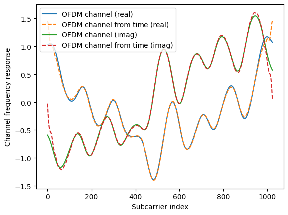
sionna.channel.time_to_ofdm_channel(h_t, rg, l_min)

Compute the channel frequency response from the discrete complex-baseband channel impulse response.

Given a discrete complex-baseband channel impulse response \(\bar{h}_{b,\ell}\), for \(\ell\) ranging from \(L_\text{min}\le 0\) to \(L_\text{max}\), the discrete channel frequency response is computed as

\[\hat{h}_{b,n} = \sum_{k=0}^{L_\text{max}} \bar{h}_{b,k} e^{-j \frac{2\pi kn}{N}} + \sum_{k=L_\text{min}}^{-1} \bar{h}_{b,k} e^{-j \frac{2\pi n(N+k)}{N}}, \quad n=0,\dots,N-1\]

where \(N\) is the FFT size and \(b\) is the time step.

This function only produces one channel frequency response per OFDM symbol, i.e., only values of \(b\) corresponding to the start of an OFDM symbol (after cyclic prefix removal) are considered.

Input

• h_t ([…num_time_steps,l_max-l_min+1], tf.complex) – Tensor of discrete complex-baseband channel impulse responses

• resource_grid (ResourceGrid) – Resource grid

• l_min (int) – Smallest time-lag for the discrete complex baseband channel impulse response (\(L_{\text{min}}\))

Output

h_f ([…,num_ofdm_symbols,fft_size], tf.complex) – Tensor of discrete complex-baseband channel frequency responses

Note

Note that the result of this function is generally different from the output of cir_to_ofdm_channel() because the discrete complex-baseband channel impulse response is truncated (see cir_to_time_channel()). This effect can be observed in the example below.

Examples

# Setup resource grid and channel model
tf.random.set_seed(4)
sm = StreamManagement(np.array([[1]]), 1)
rg = ResourceGrid(num_ofdm_symbols=1,
                  fft_size=1024,
                  subcarrier_spacing=15e3)
tdl = TDL("A", 100e-9, 3.5e9)

# Generate CIR
cir = tdl(batch_size=1, num_time_steps=1, sampling_frequency=rg.bandwidth)

# Generate OFDM channel from CIR
frequencies = subcarrier_frequencies(rg.fft_size, rg.subcarrier_spacing)
h_freq = tf.squeeze(cir_to_ofdm_channel(frequencies, *cir, normalize=True))

# Generate time channel from CIR
l_min, l_max = time_lag_discrete_time_channel(rg.bandwidth)
h_time = cir_to_time_channel(rg.bandwidth, *cir, l_min=l_min, l_max=l_max, normalize=True)

# Generate OFDM channel from time channel
h_freq_hat = tf.squeeze(time_to_ofdm_channel(h_time, rg, l_min))

# Visualize results
plt.figure()
plt.plot(np.real(h_freq), "-")
plt.plot(np.real(h_freq_hat), "--")
plt.plot(np.imag(h_freq), "-")
plt.plot(np.imag(h_freq_hat), "--")
plt.xlabel("Subcarrier index")
plt.ylabel(r"Channel frequency response")
plt.legend(["OFDM Channel (real)", "OFDM Channel from time (real)", "OFDM Channel (imag)", "OFDM Channel from time (imag)"])

Channel with OFDM waveform

To implement the channel response assuming an OFDM waveform, it is assumed that the power delay profiles are invariant over the duration of an OFDM symbol. Moreover, it is assumed that the duration of the cyclic prefix (CP) equals at least the maximum delay spread. These assumptions are common in the literature, as they enable modeling of the channel transfer function in the frequency domain as a single-tap channel.

For every link \((u, k, v, l)\) and resource element \((s,n)\), the frequency channel response is obtained by computing the Fourier transform of the channel response at the subcarrier frequencies, i.e.,

\[\begin{split}\begin{align} \widehat{h}_{u, k, v, l, s, n} &= \int_{-\infty}^{+\infty} h_{u, k, v, l}(s,\tau) e^{-j2\pi n \Delta_f \tau} d\tau\\ &= \sum_{m=0}^{M-1} a_{u, k, v, l, m}(s) e^{-j2\pi n \Delta_f \tau_{u, k, v, l, m}} \end{align}\end{split}\]

where \(s\) is used as time step to indicate that the channel response can change from one OFDM symbol to the next in the event of mobility, even if it is assumed static over the duration of an OFDM symbol.

For every receive antenna \(l\) of every receiver \(v\), the received signal \(y_{v, l, s, n}\) for resource element \((s, n)\) is computed by

\[y_{v, l, s, n} = \sum_{u=0}^{N_{T}-1}\sum_{k=0}^{N_{TA}-1} \widehat{h}_{u, k, v, l, s, n} x_{u, k, s, n} + w_{v, l, s, n}\]

where \(x_{u, k, s, n}\) is the baseband symbol transmitted by transmitter \(u\) on antenna \(k\) and resource element \((s, n)\), and \(w_{v, l, s, n} \sim \mathcal{CN}\left(0,N_0\right)\) the additive white Gaussian noise.

Note

This model does not account for intersymbol interference (ISI) nor intercarrier interference (ICI). To model the ICI due to channel aging over the duration of an OFDM symbol or the ISI due to a delay spread exceeding the CP duration, one would need to simulate the channel in the time domain. This can be achieved by using the OFDMModulator and OFDMDemodulator layers, and the time domain channel model. By doing so, one performs inverse discrete Fourier transform (IDFT) on the transmitter side and discrete Fourier transform (DFT) on the receiver side on top of a single-carrier sinc-shaped waveform. This is equivalent to simulating the channel in the frequency domain if no ISI nor ICI is assumed, but allows the simulation of these effects in the event of a non-stationary channel or long delay spreads. Note that simulating the channel in the time domain is typically significantly more computationally demanding that simulating the channel in the frequency domain.

OFDMChannel

class sionna.channel.OFDMChannel(channel_model, resource_grid, add_awgn=True, normalize_channel=False, return_channel=False, dtype=tf.complex64, **kwargs)

Generate channel frequency responses and apply them to channel inputs assuming an OFDM waveform with no ICI nor ISI.

This class inherits from the Keras Layer class and can be used as layer in a Keras model.

For each OFDM symbol \(s\) and subcarrier \(n\), the channel output is computed as follows:

\[y_{s,n} = \widehat{h}_{s, n} x_{s,n} + w_{s,n}\]

where \(y_{s,n}\) is the channel output computed by this layer, \(\widehat{h}_{s, n}\) the frequency channel response, \(x_{s,n}\) the channel input x, and \(w_{s,n}\) the additive noise.

For multiple-input multiple-output (MIMO) links, the channel output is computed for each antenna of each receiver and by summing over all the antennas of all transmitters.

The channel frequency response for the \(s^{th}\) OFDM symbol and \(n^{th}\) subcarrier is computed from a given channel impulse response \((a_{m}(t), \tau_{m}), 0 \leq m \leq M-1\) generated by the channel_model as follows:

\[\widehat{h}_{s, n} = \sum_{m=0}^{M-1} a_{m}(s) e^{-j2\pi n \Delta_f \tau_{m}}\]

where \(\Delta_f\) is the subcarrier spacing, and \(s\) is used as time step to indicate that the channel impulse response can change from one OFDM symbol to the next in the event of mobility, even if it is assumed static over the duration of an OFDM symbol.

Parameters

• channel_model (ChannelModel object) – An instance of a ChannelModel object, such as RayleighBlockFading or UMi.

• resource_grid (ResourceGrid) – Resource grid

• add_awgn (bool) – If set to False, no white Gaussian noise is added. Defaults to True.

• normalize_channel (bool) – If set to True, the channel is normalized over the resource grid to ensure unit average energy per resource element. Defaults to False.

• return_channel (bool) – If set to True, the channel response is returned in addition to the channel output. Defaults to False.

• dtype (tf.DType) – Complex datatype to use for internal processing and output. Defaults to tf.complex64.

Input

• (x, no) or x – Tuple or Tensor:

• x ([batch size, num_tx, num_tx_ant, num_ofdm_symbols, fft_size], tf.complex) – Channel inputs

• no (Scalar or Tensor, tf.float) – Scalar or tensor whose shape can be broadcast to the shape of the channel outputs: [batch size, num_rx, num_rx_ant, num_ofdm_symbols, fft_size]. Only required if add_awgn is set to True. The noise power no is per complex dimension. If no is a scalar, noise of the same variance will be added to the outputs. If no is a tensor, it must have a shape that can be broadcast to the shape of the channel outputs. This allows, e.g., adding noise of different variance to each example in a batch. If no has a lower rank than the channel outputs, then no will be broadcast to the shape of the channel outputs by adding dummy dimensions after the last axis.

Output

• y ([batch size, num_rx, num_rx_ant, num_ofdm_symbols, fft_size], tf.complex) – Channel outputs

• h_freq ([batch size, num_rx, num_rx_ant, num_tx, num_tx_ant, num_ofdm_symbols, fft_size], tf.complex) – (Optional) Channel frequency responses. Returned only if return_channel is set to True.

GenerateOFDMChannel

class sionna.channel.GenerateOFDMChannel(channel_model, resource_grid, normalize_channel=False)

Generate channel frequency responses. The channel impulse response is constant over the duration of an OFDM symbol.

Given a channel impulse response \((a_{m}(t), \tau_{m}), 0 \leq m \leq M-1\), generated by the channel_model, the channel frequency response for the \(s^{th}\) OFDM symbol and \(n^{th}\) subcarrier is computed as follows:

\[\widehat{h}_{s, n} = \sum_{m=0}^{M-1} a_{m}(s) e^{-j2\pi n \Delta_f \tau_{m}}\]

where \(\Delta_f\) is the subcarrier spacing, and \(s\) is used as time step to indicate that the channel impulse response can change from one OFDM symbol to the next in the event of mobility, even if it is assumed static over the duration of an OFDM symbol.

Parameters

• channel_model (ChannelModel object) – An instance of a ChannelModel object, such as RayleighBlockFading or UMi.

• resource_grid (ResourceGrid) – Resource grid

• normalize_channel (bool) – If set to True, the channel is normalized over the resource grid to ensure unit average energy per resource element. Defaults to False.

• dtype (tf.DType) – Complex datatype to use for internal processing and output. Defaults to tf.complex64.

Input

batch_size (int) – Batch size. Defaults to None for channel models that do not require this paranmeter.

Output

h_freq ([batch size, num_rx, num_rx_ant, num_tx, num_tx_ant, num_ofdm_symbols, num_subcarriers], tf.complex) – Channel frequency responses

ApplyOFDMChannel

class sionna.channel.ApplyOFDMChannel(add_awgn=True, dtype=tf.complex64, **kwargs)

Apply single-tap channel frequency responses to channel inputs.

This class inherits from the Keras Layer class and can be used as layer in a Keras model.

For each OFDM symbol \(s\) and subcarrier \(n\), the single-tap channel is applied as follows:

\[y_{s,n} = \widehat{h}_{s, n} x_{s,n} + w_{s,n}\]

where \(y_{s,n}\) is the channel output computed by this layer, \(\widehat{h}_{s, n}\) the frequency channel response (h_freq), \(x_{s,n}\) the channel input x, and \(w_{s,n}\) the additive noise.

For multiple-input multiple-output (MIMO) links, the channel output is computed for each antenna of each receiver and by summing over all the antennas of all transmitters.

Parameters

• add_awgn (bool) – If set to False, no white Gaussian noise is added. Defaults to True.

• dtype (tf.DType) – Complex datatype to use for internal processing and output. Defaults to tf.complex64.

Input

• (x, h_freq, no) or (x, h_freq) – Tuple:

• x ([batch size, num_tx, num_tx_ant, num_ofdm_symbols, fft_size], tf.complex) – Channel inputs

• h_freq ([batch size, num_rx, num_rx_ant, num_tx, num_tx_ant, num_ofdm_symbols, fft_size], tf.complex) – Channel frequency responses

• no (Scalar or Tensor, tf.float) – Scalar or tensor whose shape can be broadcast to the shape of the channel outputs: [batch size, num_rx, num_rx_ant, num_ofdm_symbols, fft_size]. Only required if add_awgn is set to True. The noise power no is per complex dimension. If no is a scalar, noise of the same variance will be added to the outputs. If no is a tensor, it must have a shape that can be broadcast to the shape of the channel outputs. This allows, e.g., adding noise of different variance to each example in a batch. If no has a lower rank than the channel outputs, then no will be broadcast to the shape of the channel outputs by adding dummy dimensions after the last axis.

Output

y ([batch size, num_rx, num_rx_ant, num_ofdm_symbols, fft_size], tf.complex) – Channel outputs

cir_to_ofdm_channel

sionna.channel.cir_to_ofdm_channel(frequencies, a, tau, normalize=False)

Compute the frequency response of the channel at frequencies.

Given a channel impulse response \((a_{m}, \tau_{m}), 0 \leq m \leq M-1\) (inputs a and tau), the channel frequency response for the frequency \(f\) is computed as follows:

\[\widehat{h}(f) = \sum_{m=0}^{M-1} a_{m} e^{-j2\pi f \tau_{m}}\]

Input

• frequencies ([fft_size], tf.float) – Frequencies at which to compute the channel response

• a ([batch size, num_rx, num_rx_ant, num_tx, num_tx_ant, num_paths, num_time_steps], tf.complex) – Path coefficients

• tau ([batch size, num_rx, num_tx, num_paths] or [batch size, num_rx, num_rx_ant, num_tx, num_tx_ant, num_paths], tf.float) – Path delays

• normalize (bool) – If set to True, the channel is normalized over the resource grid to ensure unit average energy per resource element. Defaults to False.

Output

h_f ([batch size, num_rx, num_rx_ant, num_tx, num_tx_ant, num_time_steps, fft_size], tf.complex) – Channel frequency responses at frequencies

Rayleigh block fading

class sionna.channel.RayleighBlockFading(num_rx, num_rx_ant, num_tx, num_tx_ant, dtype=tf.complex64)

Generate channel impulse responses corresponding to a Rayleigh block fading channel model.

The channel impulse responses generated are formed of a single path with zero delay and a normally distributed fading coefficient. All time steps of a batch example share the same channel coefficient (block fading).

This class can be used in conjunction with the classes that simulate the channel response in time or frequency domain, i.e., OFDMChannel, TimeChannel, GenerateOFDMChannel, ApplyOFDMChannel, GenerateTimeChannel, ApplyTimeChannel.

Parameters

• num_rx (int) – Number of receivers (\(N_R\))

• num_rx_ant (int) – Number of antennas per receiver (\(N_{RA}\))

• num_tx (int) – Number of transmitters (\(N_T\))

• num_tx_ant (int) – Number of antennas per transmitter (\(N_{TA}\))

• dtype (tf.DType) – Complex datatype to use for internal processing and output. Defaults to tf.complex64.

Input

• batch_size (int) – Batch size

• num_time_steps (int) – Number of time steps

Output

• a ([batch size, num_rx, num_rx_ant, num_tx, num_tx_ant, num_paths = 1, num_time_steps], tf.complex) – Path coefficients

• tau ([batch size, num_rx, num_tx, num_paths = 1], tf.float) – Path delays [s]

3GPP 38.901 channel models

The submodule tr38901 implements 3GPP channel models from [TR38901].

The CDL, UMi, UMa, and RMa models require setting-up antenna models for the transmitters and receivers. This is achieved using the PanelArray class.

The UMi, UMa, and RMa models require setting-up a network topology, specifying, e.g., the user terminals (UTs) and base stations (BSs) locations, the UTs velocities, etc. Utility functions are available to help laying out complex topologies or to quickly setup simple but widely used topologies.

PanelArray

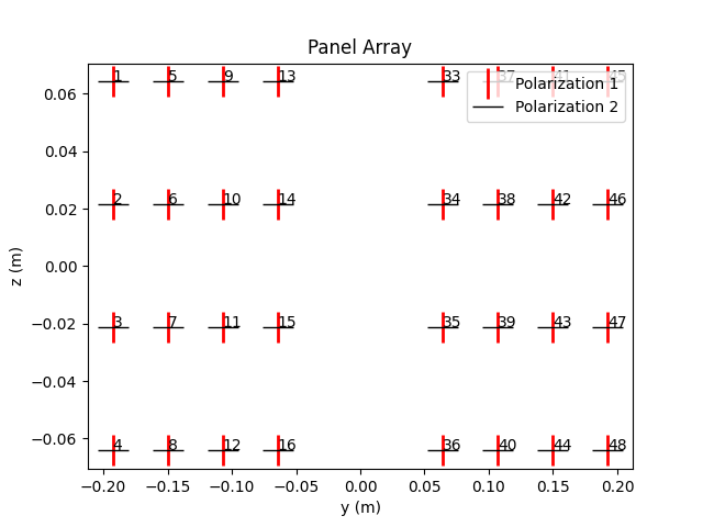
class sionna.channel.tr38901.PanelArray(num_rows_per_panel, num_cols_per_panel, polarization, polarization_type, antenna_pattern, carrier_frequency, num_rows=1, num_cols=1, panel_vertical_spacing=None, panel_horizontal_spacing=None, element_vertical_spacing=None, element_horizontal_spacing=None, dtype=tf.complex64)

Antenna panel array following the [TR38901] specification.

This class is used to create models of the panel arrays used by the transmitters and receivers and that need to be specified when using the CDL, UMi, UMa, and RMa models.

Example

>>> array = PanelArray(num_rows_per_panel = 4,
...                    num_cols_per_panel = 4,
...                    polarization = 'dual',
...                    polarization_type = 'VH',
...                    antenna_pattern = '38.901',
...                    carrier_frequency = 3.5e9,
...                    num_cols = 2,
...                    panel_horizontal_spacing = 3.)
>>> array.show()

Parameters

• num_rows_per_panel (int) – Number of rows of elements per panel

• num_cols_per_panel (int) – Number of columns of elements per panel

• polarization (str) – Polarization, either “single” or “dual”

• polarization_type (str) – Type of polarization. For single polarization, must be “V” or “H”. For dual polarization, must be “VH” or “cross”.

• antenna_pattern (str) – Element radiation pattern, either “omni” or “38.901”

• carrier_frequency (float) – Carrier frequency [Hz]

• num_rows (int) – Number of rows of panels. Defaults to 1.

• num_cols (int) – Number of columns of panels. Defaults to 1.

• panel_vertical_spacing (None or float) – Vertical spacing of panels [multiples of wavelength]. Must be greater than the panel width. If set to None (default value), it is set to the panel width + 0.5.

• panel_horizontal_spacing (None or float) – Horizontal spacing of panels [in multiples of wavelength]. Must be greater than the panel height. If set to None (default value), it is set to the panel height + 0.5.

• element_vertical_spacing (None or float) – Element vertical spacing [multiple of wavelength]. Defaults to 0.5 if set to None.

• element_horizontal_spacing (None or float) – Element horizontal spacing [multiple of wavelength]. Defaults to 0.5 if set to None.

• dtype (Complex tf.DType) – Defines the datatype for internal calculations and the output dtype. Defaults to tf.complex64.

property ant_ind_pol1

Indices of antenna elements with the first polarization direction

property ant_ind_pol2

Indices of antenna elements with the second polarization direction. Only defined with dual polarization.

property ant_pol1

Field of an antenna element with the first polarization direction

property ant_pol2

Field of an antenna element with the second polarization direction. Only defined with dual polarization.

property ant_pos

Positions of the antennas

property ant_pos_pol1

Positions of the antenna elements with the first polarization direction

property ant_pos_pol2

Positions of antenna elements with the second polarization direction. Only defined with dual polarization.

property element_horizontal_spacing

Horizontal spacing between the antenna elements within a panel [multiple of wavelength]

property element_vertical_spacing

Vertical spacing between the antenna elements within a panel [multiple of wavelength]

property num_ant

Total number of antenna elements

property num_cols

Number of columns of panels

property num_cols_per_panel

Number of columns of elements per panel

property num_panels

Number of panels

property num_panels_ant

Number of antenna elements per panel

property num_rows

Number of rows of panels

property num_rows_per_panel

Number of rows of elements per panel

property panel_horizontal_spacing

Horizontal spacing between the panels [multiple of wavelength]

property panel_vertical_spacing

Vertical spacing between the panels [multiple of wavelength]

property polarization

Polarization (“single” or “dual”)

property polarization_type

Polarization type. “V” or “H” for single polarization. “VH” or “cross” for dual polarization.

show()

Show the panel array geometry

show_element_radiation_pattern()

Show the radiation field of antenna elements forming the panel

Antenna

class sionna.channel.tr38901.Antenna(polarization, polarization_type, antenna_pattern, carrier_frequency, dtype=tf.complex64)

Single antenna following the [TR38901] specification.

This class is a special case of PanelArray, and can be used in lieu of it.

Parameters

• polarization (str) – Polarization, either “single” or “dual”

• polarization_type (str) – Type of polarization. For single polarization, must be “V” or “H”. For dual polarization, must be “VH” or “cross”.

• antenna_pattern (str) – Element radiation pattern, either “omni” or “38.901”

• carrier_frequency (float) – Carrier frequency [Hz]

• dtype (Complex tf.DType) – Defines the datatype for internal calculations and the output dtype. Defaults to tf.complex64.

AntennaArray

class sionna.channel.tr38901.AntennaArray(num_rows, num_cols, polarization, polarization_type, antenna_pattern, carrier_frequency, vertical_spacing, horizontal_spacing, dtype=tf.complex64)

Antenna array following the [TR38901] specification.

This class is a special case of PanelArray, and can used in lieu of it.

Parameters

• num_rows (int) – Number of rows of elements

• num_cols (int) – Number of columns of elements

• polarization (str) – Polarization, either “single” or “dual”

• polarization_type (str) – Type of polarization. For single polarization, must be “V” or “H”. For dual polarization, must be “VH” or “cross”.

• antenna_pattern (str) – Element radiation pattern, either “omni” or “38.901”

• carrier_frequency (float) – Carrier frequency [Hz]

• vertical_spacing (None or float) – Element vertical spacing [multiple of wavelength]. Defaults to 0.5 if set to None.

• horizontal_spacing (None or float) – Element horizontal spacing [multiple of wavelength]. Defaults to 0.5 if set to None.

• dtype (Complex tf.DType) – Defines the datatype for internal calculations and the output dtype. Defaults to tf.complex64.

Tapped delay line (TDL)

class sionna.channel.tr38901.TDL(model, delay_spread, carrier_frequency, num_sinusoids=20, los_angle_of_arrival=PI / 4., min_speed=0., max_speed=None, num_rx_ant=1, num_tx_ant=1, spatial_corr_mat=None, rx_corr_mat=None, tx_corr_mat=None, dtype=tf.complex64)

Tapped delay line (TDL) channel model from the 3GPP [TR38901] specification.

The power delay profiles (PDPs) are normalized to have a total energy of one.

Channel coefficients are generated using a sum-of-sinusoids model [SoS]. Channel aging is simulated in the event of mobility.

If a minimum speed and a maximum speed are specified such that the maximum speed is greater than the minimum speed, then speeds are randomly and uniformly sampled from the specified interval for each link and each batch example.

The TDL model only works for systems with a single transmitter and a single receiver. The transmitter and receiver can be equipped with multiple antennas. Spatial correlation is simulated through filtering by specified correlation matrices.

The spatial_corr_mat parameter can be used to specify an arbitrary spatial correlation matrix. In particular, it can be used to model correlated cross-polarized transmit and receive antennas as follows (see, e.g., Annex G.2.3.2.1 [TS38141-1]):

\[\mathbf{R} = \mathbf{R}_{\text{rx}} \otimes \mathbf{\Gamma} \otimes \mathbf{R}_{\text{tx}}\]

where \(\mathbf{R}\) is the spatial correlation matrix spatial_corr_mat, \(\mathbf{R}_{\text{rx}}\) the spatial correlation matrix at the receiver with same polarization, \(\mathbf{R}_{\text{tx}}\) the spatial correlation matrix at the transmitter with same polarization, and \(\mathbf{\Gamma}\) the polarization correlation matrix. \(\mathbf{\Gamma}\) is 1x1 for single-polarized antennas, 2x2 when only the transmit or receive antennas are cross-polarized, and 4x4 when transmit and receive antennas are cross-polarized.

It is also possible not to specify spatial_corr_mat, but instead the correlation matrices at the receiver and transmitter, using the rx_corr_mat and tx_corr_mat parameters, respectively. This can be useful when single polarized antennas are simulated, and it is also more computationally efficient. This is equivalent to setting spatial_corr_mat to :

\[\mathbf{R} = \mathbf{R}_{\text{rx}} \otimes \mathbf{R}_{\text{tx}}\]

where \(\mathbf{R}_{\text{rx}}\) is the correlation matrix at the receiver rx_corr_mat and \(\mathbf{R}_{\text{tx}}\) the correlation matrix at the transmitter tx_corr_mat.

Example

The following code snippet shows how to setup a TDL channel model assuming an OFDM waveform:

>>> tdl = TDL(model = "A",
...           delay_spread = 300e-9,
...           carrier_frequency = 3.5e9,
...           min_speed = 0.0,
...           max_speed = 3.0)
>>>
>>> channel = OFDMChannel(channel_model = tdl,
...                       resource_grid = rg)

where rg is an instance of ResourceGrid.

Notes

The following tables from [TR38901] provide typical values for the delay spread.

Model	Delay spread [ns]
Very short delay spread	\(10\)
Short short delay spread	\(10\)
Nominal delay spread	\(100\)
Long delay spread	\(300\)
Very long delay spread	\(1000\)

Delay spread [ns]		Frequency [GHz]
		2	6	15	28	39	60	70
Indoor office	Short delay profile	20	16	16	16	16	16	16
	Normal delay profile	39	30	24	20	18	16	16
	Long delay profile	59	53	47	43	41	38	37
UMi Street-canyon	Short delay profile	65	45	37	32	30	27	26
	Normal delay profile	129	93	76	66	61	55	53
	Long delay profile	634	316	307	301	297	293	291
UMa	Short delay profile	93	93	85	80	78	75	74
	Normal delay profile	363	363	302	266	249	228	221
	Long delay profile	1148	1148	955	841	786	720	698
RMa / RMa O2I	Short delay profile	32	32	N/A	N/A	N/A	N/A	N/A
	Normal delay profile	37	37	N/A	N/A	N/A	N/A	N/A
	Long delay profile	153	153	N/A	N/A	N/A	N/A	N/A
UMi / UMa O2I	Normal delay profile	242
	Long delay profile	616

Parameters

• model (str) – TDL model to use. Must be one of “A”, “B”, “C”, “D”, “E”, “A30”, “B100”, or “C300”.

• delay_spread (float) – RMS delay spread [s]. For the “A30”, “B100”, and “C300” models, the delay spread must be set to 30ns, 100ns, and 300ns, respectively.

• carrier_frequency (float) – Carrier frequency [Hz]

• num_sinusoids (int) – Number of sinusoids for the sum-of-sinusoids model. Defaults to 20.

• los_angle_of_arrival (float) – Angle-of-arrival for LoS path [radian]. Only used with LoS models. Defaults to \(\pi/4\).

• min_speed (float) – Minimum speed [m/s]. Defaults to 0.

• max_speed (None or float) – Maximum speed [m/s]. If set to None, then max_speed takes the same value as min_speed. Defaults to None.

• num_rx_ant (int) – Number of receive antennas. Defaults to 1.

• num_tx_ant (int) – Number of transmit antennas. Defaults to 1.

• spatial_corr_mat ([num_rx_ant*num_tx_ant,num_rx_ant*num_tx_ant], tf.complex or None) – Spatial correlation matrix. If not set to None, then rx_corr_mat and tx_corr_mat are ignored and this matrix is used for spatial correlation. If set to None and rx_corr_mat and tx_corr_mat are also set to None, then no correlation is applied. Defaults to None.

• rx_corr_mat ([num_rx_ant,num_rx_ant], tf.complex or None) – Spatial correlation matrix for the receiver. If set to None and spatial_corr_mat is also set to None, then no receive correlation is applied. Defaults to None.

• tx_corr_mat ([num_tx_ant,num_tx_ant], tf.complex or None) – Spatial correlation matrix for the transmitter. If set to None and spatial_corr_mat is also set to None, then no transmit correlation is applied. Defaults to None.

• dtype (Complex tf.DType) – Defines the datatype for internal calculations and the output dtype. Defaults to tf.complex64.

Input

• batch_size (int) – Batch size

• num_time_steps (int) – Number of time steps

• sampling_frequency (float) – Sampling frequency [Hz]

Output

• a ([batch size, num_rx = 1, num_rx_ant = 1, num_tx = 1, num_tx_ant = 1, num_paths, num_time_steps], tf.complex) – Path coefficients

• tau ([batch size, num_rx = 1, num_tx = 1, num_paths], tf.float) – Path delays [s]

property delay_spread

RMS delay spread [s]

property delays

Path delays [s]

property k_factor

K-factor in linear scale. Only available with LoS models.

property los

True if this is a LoS model. False otherwise.

property mean_power_los

LoS component power in linear scale. Only available with LoS models.

property mean_powers

Path powers in linear scale

property num_clusters

Number of paths (\(M\))

Clustered delay line (CDL)

class sionna.channel.tr38901.CDL(model, delay_spread, carrier_frequency, ut_array, bs_array, direction, min_speed=0., max_speed=None, dtype=tf.complex64)

Clustered delay line (CDL) channel model from the 3GPP [TR38901] specification.

The power delay profiles (PDPs) are normalized to have a total energy of one.

If a minimum speed and a maximum speed are specified such that the maximum speed is greater than the minimum speed, then UTs speeds are randomly and uniformly sampled from the specified interval for each link and each batch example.

The CDL model only works for systems with a single transmitter and a single receiver. The transmitter and receiver can be equipped with multiple antennas.

Example

The following code snippet shows how to setup a CDL channel model assuming an OFDM waveform:

>>> # Panel array configuration for the transmitter and receiver
>>> bs_array = PanelArray(num_rows_per_panel = 4,
...                       num_cols_per_panel = 4,
...                       polarization = 'dual',
...                       polarization_type = 'cross',
...                       antenna_pattern = '38.901',
...                       carrier_frequency = 3.5e9)
>>> ut_array = PanelArray(num_rows_per_panel = 1,
...                       num_cols_per_panel = 1,
...                       polarization = 'single',
...                       polarization_type = 'V',
...                       antenna_pattern = 'omni',
...                       carrier_frequency = 3.5e9)
>>> # CDL channel model
>>> cdl = CDL(model = "A",
>>>           delay_spread = 300e-9,
...           carrier_frequency = 3.5e9,
...           ut_array = ut_array,
...           bs_array = bs_array,
...           direction = 'uplink')
>>> channel = OFDMChannel(channel_model = cdl,
...                       resource_grid = rg)

where rg is an instance of ResourceGrid.

Notes

The following tables from [TR38901] provide typical values for the delay spread.

Model	Delay spread [ns]
Very short delay spread	\(10\)
Short short delay spread	\(10\)
Nominal delay spread	\(100\)
Long delay spread	\(300\)
Very long delay spread	\(1000\)

Delay spread [ns]		Frequency [GHz]
		2	6	15	28	39	60	70
Indoor office	Short delay profile	20	16	16	16	16	16	16
	Normal delay profile	39	30	24	20	18	16	16
	Long delay profile	59	53	47	43	41	38	37
UMi Street-canyon	Short delay profile	65	45	37	32	30	27	26
	Normal delay profile	129	93	76	66	61	55	53
	Long delay profile	634	316	307	301	297	293	291
UMa	Short delay profile	93	93	85	80	78	75	74
	Normal delay profile	363	363	302	266	249	228	221
	Long delay profile	1148	1148	955	841	786	720	698
RMa / RMa O2I	Short delay profile	32	32	N/A	N/A	N/A	N/A	N/A
	Normal delay profile	37	37	N/A	N/A	N/A	N/A	N/A
	Long delay profile	153	153	N/A	N/A	N/A	N/A	N/A
UMi / UMa O2I	Normal delay profile	242
	Long delay profile	616

Parameters

• model (str) – CDL model to use. Must be one of “A”, “B”, “C”, “D” or “E”.

• delay_spread (float) – RMS delay spread [s].

• carrier_frequency (float) – Carrier frequency [Hz].

• ut_array (PanelArray) – Panel array used by the UTs. All UTs share the same antenna array configuration.

• bs_array (PanelArray) – Panel array used by the Bs. All BSs share the same antenna array configuration.

• direction (str) – Link direction. Must be either “uplink” or “downlink”.

• ut_orientation (None or Tensor of shape [3], tf.float) – Orientation of the UT. If set to None, [\(\pi\), 0, 0] is used. Defaults to None.

• bs_orientation (None or Tensor of shape [3], tf.float) – Orientation of the BS. If set to None, [0, 0, 0] is used. Defaults to None.

• min_speed (float) – Minimum speed [m/s]. Defaults to 0.

• max_speed (None or float) – Maximum speed [m/s]. If set to None, then max_speed takes the same value as min_speed. Defaults to None.

• dtype (Complex tf.DType) – Defines the datatype for internal calculations and the output dtype. Defaults to tf.complex64.

Input

• batch_size (int) – Batch size

• num_time_steps (int) – Number of time steps

• sampling_frequency (float) – Sampling frequency [Hz]

Output

• a ([batch size, num_rx = 1, num_rx_ant, num_tx = 1, num_tx_ant, num_paths, num_time_steps], tf.complex) – Path coefficients

• tau ([batch size, num_rx = 1, num_tx = 1, num_paths], tf.float) – Path delays [s]

property delay_spread

RMS delay spread [s]

property delays

Path delays [s]

property k_factor

K-factor in linear scale. Only available with LoS models.

property los

True is this is a LoS model. False otherwise.

property num_clusters

Number of paths (\(M\))

property powers

Path powers in linear scale

Urban microcell (UMi)

class sionna.channel.tr38901.UMi(carrier_frequency, o2i_model, ut_array, bs_array, direction, enable_pathloss=True, enable_shadow_fading=True, always_generate_lsp=False, dtype=tf.complex64)

Urban microcell (UMi) channel model from 3GPP [TR38901] specification.

Setting up a UMi model requires configuring the network topology, i.e., the UTs and BSs locations, UTs velocities, etc. This is achieved using the set_topology() method. Setting a different topology for each batch example is possible. The batch size used when setting up the network topology is used for the link simulations.

The following code snippet shows how to setup a UMi channel model operating in the frequency domain:

>>> # UT and BS panel arrays
>>> bs_array = PanelArray(num_rows_per_panel = 4,
...                       num_cols_per_panel = 4,
...                       polarization = 'dual',
...                       polarization_type  = 'cross',
...                       antenna_pattern = '38.901',
...                       carrier_frequency = 3.5e9)
>>> ut_array = PanelArray(num_rows_per_panel = 1,
...                       num_cols_per_panel = 1,
...                       polarization = 'single',
...                       polarization_type = 'V',
...                       antenna_pattern = 'omni',
...                       carrier_frequency = 3.5e9)
>>> # Instantiating UMi channel model
>>> channel_model = UMi(carrier_frequency = 3.5e9,
...                     o2i_model = 'low',
...                     ut_array = ut_array,
...                     bs_array = bs_array,
...                     direction = 'uplink')
>>> # Setting up network topology
>>> # ut_loc: UTs locations
>>> # bs_loc: BSs locations
>>> # ut_orientations: UTs array orientations
>>> # bs_orientations: BSs array orientations
>>> # in_state: Indoor/outdoor states of UTs
>>> channel_model.set_topology(ut_loc,
...                            bs_loc,
...                            ut_orientations,
...                            bs_orientations,
...                            ut_velocities,
...                            in_state)
>>> # Instanting the frequency domain channel
>>> channel = OFDMChannel(channel_model = channel_model,
...                       resource_grid = rg)

where rg is an instance of ResourceGrid.

Parameters

• carrier_frequency (float) – Carrier frequency in Hertz

• o2i_model (str) – Outdoor-to-indoor loss model for UTs located indoor. Set this parameter to “low” to use the low-loss model, or to “high” to use the high-loss model. See section 7.4.3 of [TR38901] for details.

• rx_array (PanelArray) – Panel array used by the receivers. All receivers share the same antenna array configuration.

• tx_array (PanelArray) – Panel array used by the transmitters. All transmitters share the same antenna array configuration.

• direction (str) – Link direction. Either “uplink” or “downlink”.

• enable_pathloss (bool) – If True, apply pathloss. Otherwise doesn’t. Defaults to True.

• enable_shadow_fading (bool) – If True, apply shadow fading. Otherwise doesn’t. Defaults to True.

• always_generate_lsp (bool) – If True, new large scale parameters (LSPs) are generated for every new generation of channel impulse responses. Otherwise, always reuse the same LSPs, except if the topology is changed. Defaults to False.

• dtype (Complex tf.DType) – Defines the datatype for internal calculations and the output dtype. Defaults to tf.complex64.

Input

• num_time_steps (int) – Number of time steps

• sampling_frequency (float) – Sampling frequency [Hz]

Output

• a ([batch size, num_rx, num_rx_ant, num_tx, num_tx_ant, num_paths, num_time_steps], tf.complex) – Path coefficients

• tau ([batch size, num_rx, num_tx, num_paths], tf.float) – Path delays [s]

set_topology(ut_loc=None, bs_loc=None, ut_orientations=None, bs_orientations=None, ut_velocities=None, in_state=None, los=None)

Set the network topology.

It is possible to set up a different network topology for each batch example. The batch size used when setting up the network topology is used for the link simulations.

When calling this function, not specifying a parameter leads to the reuse of the previously given value. Not specifying a value that was not set at a former call rises an error.

Input

• ut_loc ([batch size,num_ut, 3], tf.float) – Locations of the UTs

• bs_loc ([batch size,num_bs, 3], tf.float) – Locations of BSs

• ut_orientations ([batch size,num_ut, 3], tf.float) – Orientations of the UTs arrays [radian]

• bs_orientations ([batch size,num_bs, 3], tf.float) – Orientations of the BSs arrays [radian]

• ut_velocities ([batch size,num_ut, 3], tf.float) – Velocity vectors of UTs

• in_state ([batch size,num_ut], tf.bool) – Indoor/outdoor state of UTs. True means indoor and False means outdoor.

• los (tf.bool or None) – If not None (default value), all UTs located outdoor are forced to be in LoS if los is set to True, or in NLoS if it is set to False. If set to None, the LoS/NLoS states of UTs is set following 3GPP specification [TR38901].

Note

If you want to use this function in Graph mode with XLA, i.e., within a function that is decorated with @tf.function(jit_compile=True), you must set sionna.Config.xla_compat=true. See xla_compat.

show_topology(bs_index=0, batch_index=0)

Shows the network topology of the batch example with index batch_index.

The bs_index parameter specifies with respect to which BS the LoS/NLoS state of UTs is indicated.

Input

• bs_index (int) – BS index with respect to which the LoS/NLoS state of UTs is indicated. Defaults to 0.

• batch_index (int) – Batch example for which the topology is shown. Defaults to 0.

Urban macrocell (UMa)

class sionna.channel.tr38901.UMa(carrier_frequency, o2i_model, ut_array, bs_array, direction, enable_pathloss=True, enable_shadow_fading=True, always_generate_lsp=False, dtype=tf.complex64)

Urban macrocell (UMa) channel model from 3GPP [TR38901] specification.

Setting up a UMa model requires configuring the network topology, i.e., the UTs and BSs locations, UTs velocities, etc. This is achieved using the set_topology() method. Setting a different topology for each batch example is possible. The batch size used when setting up the network topology is used for the link simulations.

The following code snippet shows how to setup an UMa channel model assuming an OFDM waveform:

>>> # UT and BS panel arrays
>>> bs_array = PanelArray(num_rows_per_panel = 4,
...                       num_cols_per_panel = 4,
...                       polarization = 'dual',
...                       polarization_type = 'cross',
...                       antenna_pattern = '38.901',
...                       carrier_frequency = 3.5e9)
>>> ut_array = PanelArray(num_rows_per_panel = 1,
...                       num_cols_per_panel = 1,
...                       polarization = 'single',
...                       polarization_type = 'V',
...                       antenna_pattern = 'omni',
...                       carrier_frequency = 3.5e9)
>>> # Instantiating UMa channel model
>>> channel_model = UMa(carrier_frequency = 3.5e9,
...                     o2i_model = 'low',
...                     ut_array = ut_array,
...                     bs_array = bs_array,
...                     direction = 'uplink')
>>> # Setting up network topology
>>> # ut_loc: UTs locations
>>> # bs_loc: BSs locations
>>> # ut_orientations: UTs array orientations
>>> # bs_orientations: BSs array orientations
>>> # in_state: Indoor/outdoor states of UTs
>>> channel_model.set_topology(ut_loc,
...                            bs_loc,
...                            ut_orientations,
...                            bs_orientations,
...                            ut_velocities,
...                            in_state)
>>> # Instanting the OFDM channel
>>> channel = OFDMChannel(channel_model = channel_model,
...                       resource_grid = rg)

where rg is an instance of ResourceGrid.

Parameters

• carrier_frequency (float) – Carrier frequency in Hertz

• o2i_model (str) – Outdoor-to-indoor loss model for UTs located indoor. Set this parameter to “low” to use the low-loss model, or to “high” to use the high-loss model. See section 7.4.3 of [TR38901] for details.

• rx_array (PanelArray) – Panel array used by the receivers. All receivers share the same antenna array configuration.

• tx_array (PanelArray) – Panel array used by the transmitters. All transmitters share the same antenna array configuration.

• direction (str) – Link direction. Either “uplink” or “downlink”.

• enable_pathloss (bool) – If True, apply pathloss. Otherwise doesn’t. Defaults to True.

• enable_shadow_fading (bool) – If True, apply shadow fading. Otherwise doesn’t. Defaults to True.

• always_generate_lsp (bool) – If True, new large scale parameters (LSPs) are generated for every new generation of channel impulse responses. Otherwise, always reuse the same LSPs, except if the topology is changed. Defaults to False.

• dtype (Complex tf.DType) – Defines the datatype for internal calculations and the output dtype. Defaults to tf.complex64.

Input

• num_time_steps (int) – Number of time steps

• sampling_frequency (float) – Sampling frequency [Hz]

Output

• a ([batch size, num_rx, num_rx_ant, num_tx, num_tx_ant, num_paths, num_time_steps], tf.complex) – Path coefficients

• tau ([batch size, num_rx, num_tx, num_paths], tf.float) – Path delays [s]

set_topology(ut_loc=None, bs_loc=None, ut_orientations=None, bs_orientations=None, ut_velocities=None, in_state=None, los=None)

Set the network topology.

It is possible to set up a different network topology for each batch example. The batch size used when setting up the network topology is used for the link simulations.

When calling this function, not specifying a parameter leads to the reuse of the previously given value. Not specifying a value that was not set at a former call rises an error.

Input

• ut_loc ([batch size,num_ut, 3], tf.float) – Locations of the UTs

• bs_loc ([batch size,num_bs, 3], tf.float) – Locations of BSs

• ut_orientations ([batch size,num_ut, 3], tf.float) – Orientations of the UTs arrays [radian]

• bs_orientations ([batch size,num_bs, 3], tf.float) – Orientations of the BSs arrays [radian]

• ut_velocities ([batch size,num_ut, 3], tf.float) – Velocity vectors of UTs

• in_state ([batch size,num_ut], tf.bool) – Indoor/outdoor state of UTs. True means indoor and False means outdoor.

• los (tf.bool or None) – If not None (default value), all UTs located outdoor are forced to be in LoS if los is set to True, or in NLoS if it is set to False. If set to None, the LoS/NLoS states of UTs is set following 3GPP specification [TR38901].

Note

If you want to use this function in Graph mode with XLA, i.e., within a function that is decorated with @tf.function(jit_compile=True), you must set sionna.Config.xla_compat=true. See xla_compat.

show_topology(bs_index=0, batch_index=0)

Shows the network topology of the batch example with index batch_index.

The bs_index parameter specifies with respect to which BS the LoS/NLoS state of UTs is indicated.

Input

• bs_index (int) – BS index with respect to which the LoS/NLoS state of UTs is indicated. Defaults to 0.

• batch_index (int) – Batch example for which the topology is shown. Defaults to 0.

Rural macrocell (RMa)

class sionna.channel.tr38901.RMa(carrier_frequency, ut_array, bs_array, direction, enable_pathloss=True, enable_shadow_fading=True, always_generate_lsp=False, dtype=tf.complex64)

Rural macrocell (RMa) channel model from 3GPP [TR38901] specification.

Setting up a RMa model requires configuring the network topology, i.e., the UTs and BSs locations, UTs velocities, etc. This is achieved using the set_topology() method. Setting a different topology for each batch example is possible. The batch size used when setting up the network topology is used for the link simulations.

The following code snippet shows how to setup an RMa channel model assuming an OFDM waveform:

>>> # UT and BS panel arrays
>>> bs_array = PanelArray(num_rows_per_panel = 4,
...                       num_cols_per_panel = 4,
...                       polarization = 'dual',
...                       polarization_type = 'cross',
...                       antenna_pattern = '38.901',
...                       carrier_frequency = 3.5e9)
>>> ut_array = PanelArray(num_rows_per_panel = 1,
...                       num_cols_per_panel = 1,
...                       polarization = 'single',
...                       polarization_type = 'V',
...                       antenna_pattern = 'omni',
...                       carrier_frequency = 3.5e9)
>>> # Instantiating RMa channel model
>>> channel_model = RMa(carrier_frequency = 3.5e9,
...                     ut_array = ut_array,
...                     bs_array = bs_array,
...                     direction = 'uplink')
>>> # Setting up network topology
>>> # ut_loc: UTs locations
>>> # bs_loc: BSs locations
>>> # ut_orientations: UTs array orientations
>>> # bs_orientations: BSs array orientations
>>> # in_state: Indoor/outdoor states of UTs
>>> channel_model.set_topology(ut_loc,
...                            bs_loc,
...                            ut_orientations,
...                            bs_orientations,
...                            ut_velocities,
...                            in_state)
>>> # Instanting the OFDM channel
>>> channel = OFDMChannel(channel_model = channel_model,
...                       resource_grid = rg)

where rg is an instance of ResourceGrid.

Parameters

• carrier_frequency (float) – Carrier frequency [Hz]

• rx_array (PanelArray) – Panel array used by the receivers. All receivers share the same antenna array configuration.

• tx_array (PanelArray) – Panel array used by the transmitters. All transmitters share the same antenna array configuration.

• direction (str) – Link direction. Either “uplink” or “downlink”.

• enable_pathloss (bool) – If True, apply pathloss. Otherwise doesn’t. Defaults to True.

• enable_shadow_fading (bool) – If True, apply shadow fading. Otherwise doesn’t. Defaults to True.

• average_street_width (float) – Average street width [m]. Defaults to 5m.

• average_street_width – Average building height [m]. Defaults to 20m.

• always_generate_lsp (bool) – If True, new large scale parameters (LSPs) are generated for every new generation of channel impulse responses. Otherwise, always reuse the same LSPs, except if the topology is changed. Defaults to False.

• dtype (Complex tf.DType) – Defines the datatype for internal calculations and the output dtype. Defaults to tf.complex64.

Input

• num_time_steps (int) – Number of time steps

• sampling_frequency (float) – Sampling frequency [Hz]

Output

• a ([batch size, num_rx, num_rx_ant, num_tx, num_tx_ant, num_paths, num_time_steps], tf.complex) – Path coefficients

• tau ([batch size, num_rx, num_tx, num_paths], tf.float) – Path delays [s]

set_topology(ut_loc=None, bs_loc=None, ut_orientations=None, bs_orientations=None, ut_velocities=None, in_state=None, los=None)

Set the network topology.

It is possible to set up a different network topology for each batch example. The batch size used when setting up the network topology is used for the link simulations.

When calling this function, not specifying a parameter leads to the reuse of the previously given value. Not specifying a value that was not set at a former call rises an error.

Input

• ut_loc ([batch size,num_ut, 3], tf.float) – Locations of the UTs

• bs_loc ([batch size,num_bs, 3], tf.float) – Locations of BSs

• ut_orientations ([batch size,num_ut, 3], tf.float) – Orientations of the UTs arrays [radian]

• bs_orientations ([batch size,num_bs, 3], tf.float) – Orientations of the BSs arrays [radian]

• ut_velocities ([batch size,num_ut, 3], tf.float) – Velocity vectors of UTs

• in_state ([batch size,num_ut], tf.bool) – Indoor/outdoor state of UTs. True means indoor and False means outdoor.

• los (tf.bool or None) – If not None (default value), all UTs located outdoor are forced to be in LoS if los is set to True, or in NLoS if it is set to False. If set to None, the LoS/NLoS states of UTs is set following 3GPP specification [TR38901].

Note

If you want to use this function in Graph mode with XLA, i.e., within a function that is decorated with @tf.function(jit_compile=True), you must set sionna.Config.xla_compat=true. See xla_compat.

show_topology(bs_index=0, batch_index=0)

Shows the network topology of the batch example with index batch_index.

The bs_index parameter specifies with respect to which BS the LoS/NLoS state of UTs is indicated.

Input

• bs_index (int) – BS index with respect to which the LoS/NLoS state of UTs is indicated. Defaults to 0.

• batch_index (int) – Batch example for which the topology is shown. Defaults to 0.

External datasets

class sionna.channel.CIRDataset(cir_generator, batch_size, num_rx, num_rx_ant, num_tx, num_tx_ant, num_paths, num_time_steps, dtype=tf.complex64)

Creates a channel model from a dataset that can be used with classes such as TimeChannel and OFDMChannel. The dataset is defined by a generator.

The batch size is configured when instantiating the dataset or through the batch_size property. The number of time steps (num_time_steps) and sampling frequency (sampling_frequency) can only be set when instantiating the dataset. The specified values must be in accordance with the data.

Example

The following code snippet shows how to use this class as a channel model.

>>> my_generator = MyGenerator(...)
>>> channel_model = sionna.channel.CIRDataset(my_generator,
...                                           batch_size,
...                                           num_rx,
...                                           num_rx_ant,
...                                           num_tx,
...                                           num_tx_ant,
...                                           num_paths,
...                                           num_time_steps+l_tot-1)
>>> channel = sionna.channel.TimeChannel(channel_model, bandwidth, num_time_steps)

where MyGenerator is a generator

>>> class MyGenerator:
...
...     def __call__(self):
...         ...
...         yield a, tau

that returns complex-valued path coefficients a with shape [num_rx, num_rx_ant, num_tx, num_tx_ant, num_paths, num_time_steps] and real-valued path delays tau (in second) [num_rx, num_tx, num_paths].

Parameters

• cir_generator – Generator that returns channel impulse responses (a, tau) where a is the tensor of channel coefficients of shape [num_rx, num_rx_ant, num_tx, num_tx_ant, num_paths, num_time_steps] and dtype dtype, and tau the tensor of path delays of shape [num_rx, num_tx, num_paths] and dtype dtype. real_dtype.

• batch_size (int) – Batch size

• num_rx (int) – Number of receivers (\(N_R\))

• num_rx_ant (int) – Number of antennas per receiver (\(N_{RA}\))

• num_tx (int) – Number of transmitters (\(N_T\))

• num_tx_ant (int) – Number of antennas per transmitter (\(N_{TA}\))

• num_paths (int) – Number of paths (\(M\))

• num_time_steps (int) – Number of time steps

• dtype (tf.DType) – Complex datatype to use for internal processing and output. Defaults to tf.complex64.

Output

• a ([batch size, num_rx, num_rx_ant, num_tx, num_tx_ant, num_paths, num_time_steps], tf.complex) – Path coefficients

• tau ([batch size, num_rx, num_tx, num_paths], tf.float) – Path delays [s]

property batch_size

Batch size

Utility functions

subcarrier_frequencies

sionna.channel.subcarrier_frequencies(num_subcarriers, subcarrier_spacing, dtype=tf.complex64)

Compute the baseband frequencies of num_subcarrier subcarriers spaced by subcarrier_spacing, i.e.,

>>> # If num_subcarrier is even:
>>> frequencies = [-num_subcarrier/2, ..., 0, ..., num_subcarrier/2-1] * subcarrier_spacing
>>>
>>> # If num_subcarrier is odd:
>>> frequencies = [-(num_subcarrier-1)/2, ..., 0, ..., (num_subcarrier-1)/2] * subcarrier_spacing

Input

• num_subcarriers (int) – Number of subcarriers

• subcarrier_spacing (float) – Subcarrier spacing [Hz]

• dtype (tf.DType) – Datatype to use for internal processing and output. If a complex datatype is provided, the corresponding precision of real components is used. Defaults to tf.complex64 (tf.float32).

Output

frequencies ([num_subcarrier], tf.float) – Baseband frequencies of subcarriers

time_lag_discrete_time_channel

sionna.channel.time_lag_discrete_time_channel(bandwidth, maximum_delay_spread=3e-06)

Compute the smallest and largest time-lag for the descrete complex baseband channel, i.e., \(L_{\text{min}}\) and \(L_{\text{max}}\).

The smallest time-lag (\(L_{\text{min}}\)) returned is always -6, as this value was found small enough for all models included in Sionna.

The largest time-lag (\(L_{\text{max}}\)) is computed from the bandwidth and maximum_delay_spread as follows:

\[L_{\text{max}} = \lceil W \tau_{\text{max}} \rceil + 6\]

where \(L_{\text{max}}\) is the largest time-lag, \(W\) the bandwidth, and \(\tau_{\text{max}}\) the maximum_delay_spread.

The default value for the maximum_delay_spread is 3us, which was found to be large enough to include most significant paths with all channel models included in Sionna assuming a nominal delay spread of 100ns.

Note

The values of \(L_{\text{min}}\) and \(L_{\text{max}}\) computed by this function are only recommended values. \(L_{\text{min}}\) and \(L_{\text{max}}\) should be set according to the considered channel model. For OFDM systems, one also needs to be careful that the effective length of the complex baseband channel is not larger than the cyclic prefix length.

Input

• bandwidth (float) – Bandwith (\(W\)) [Hz]

• maximum_delay_spread (float) – Maximum delay spread [s]. Defaults to 3us.

Output

• l_min (int) – Smallest time-lag (\(L_{\text{min}}\)) for the descrete complex baseband channel. Set to -6, , as this value was found small enough for all models included in Sionna.

• l_max (int) – Largest time-lag (\(L_{\text{max}}\)) for the descrete complex baseband channel

deg_2_rad

sionna.channel.deg_2_rad(x)

Convert degree to radian

Input

x (Tensor) – Angles in degree

Output

y (Tensor) – Angles x converted to radian

rad_2_deg

sionna.channel.rad_2_deg(x)

Convert radian to degree

Input

x (Tensor) – Angles in radian

Output

y (Tensor) – Angles x converted to degree

wrap_angle_0_360

sionna.channel.wrap_angle_0_360(angle)

Wrap angle to (0,360)

Input

angle (Tensor) – Input to wrap

Output

y (Tensor) – angle wrapped to (0,360)

drop_uts_in_sector

sionna.channel.drop_uts_in_sector(batch_size, num_ut, min_bs_ut_dist, isd, dtype=tf.complex64)

Uniformly sample UT locations from a sector.

The sector from which UTs are sampled is shown in the following figure. The BS is assumed to be located at the origin (0,0) of the coordinate system.

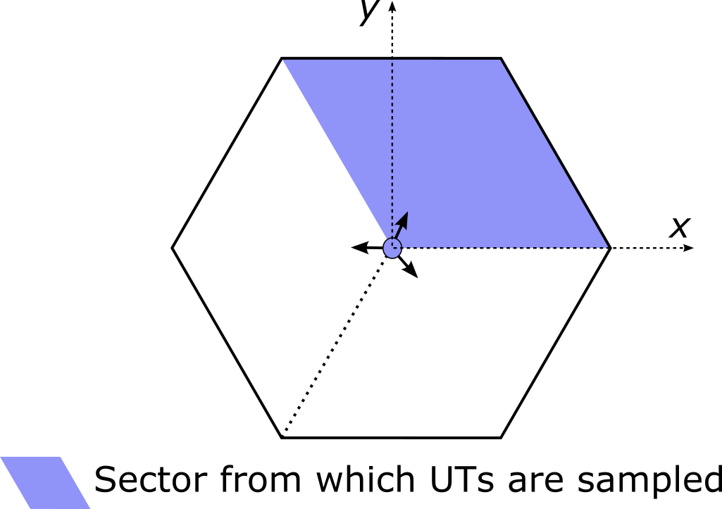
Input

• batch_size (int) – Batch size

• num_ut (int) – Number of UTs to sample per batch example

• min_bs_ut_dist (tf.float) – Minimum BS-UT distance [m]

• isd (tf.float) – Inter-site distance, i.e., the distance between two adjacent BSs [m]

• dtype (tf.DType) – Datatype to use for internal processing and output. If a complex datatype is provided, the corresponding precision of real components is used. Defaults to tf.complex64 (tf.float32).

Output

ut_loc ([batch_size, num_ut, 2], tf.float) – UTs locations in the X-Y plan

relocate_uts

sionna.channel.relocate_uts(ut_loc, sector_id, cell_loc)

Relocate the UTs by rotating them into the sector with index sector_id and transposing them to the cell centered on cell_loc.

sector_id gives the index of the sector to which the UTs are rotated to. The picture below shows how the three sectors of a cell are indexed.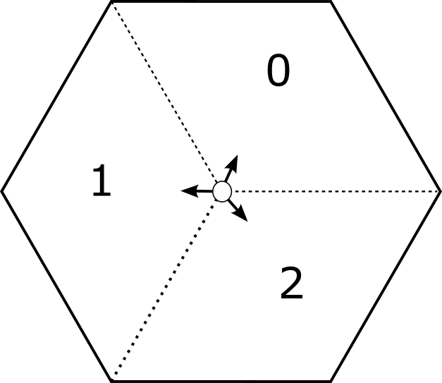

Fig. 9 Indexing of sectors

If sector_id is a scalar, then all UTs are relocated to the same sector indexed by sector_id. If sector_id is a tensor, it should be broadcastable with [batch_size, num_ut], and give the sector in which each UT or batch example is relocated to.

When calling the function, ut_loc gives the locations of the UTs to relocate, which are all assumed to be in sector with index 0, and in the cell centered on the origin (0,0).

Input

• ut_loc ([batch_size, num_ut, 2], tf.float) – UTs locations in the X-Y plan

• sector_id (Tensor broadcastable with [batch_size, num_ut], int) – Indexes of the sector to which to relocate the UTs

• cell_loc (Tensor broadcastable with [batch_size, num_ut], tf.float) – Center of the cell to which to transpose the UTs

Output

ut_loc ([batch_size, num_ut, 2], tf.float) – Relocated UTs locations in the X-Y plan

set_3gpp_scenario_parameters

sionna.channel.set_3gpp_scenario_parameters(scenario, min_bs_ut_dist=None, isd=None, bs_height=None, min_ut_height=None, max_ut_height=None, indoor_probability=None, min_ut_velocity=None, max_ut_velocity=None, dtype=tf.complex64)

Set valid parameters for a specified 3GPP system level scenario (RMa, UMi, or UMa).

If a parameter is given, then it is returned. If it is set to None, then a parameter valid according to the chosen scenario is returned (see [TR38901]).

Input

• scenario (str) – System level model scenario. Must be one of “rma”, “umi”, or “uma”.

• min_bs_ut_dist (None or tf.float) – Minimum BS-UT distance [m]

• isd (None or tf.float) – Inter-site distance [m]

• bs_height (None or tf.float) – BS elevation [m]

• min_ut_height (None or tf.float) – Minimum UT elevation [m]

• max_ut_height (None or tf.float) – Maximum UT elevation [m]

• indoor_probability (None or tf.float) – Probability of a UT to be indoor

• min_ut_velocity (None or tf.float) – Minimum UT velocity [m/s]

• max_ut_velocity (None or tf.float) – Maximim UT velocity [m/s]

• dtype (tf.DType) – Datatype to use for internal processing and output. If a complex datatype is provided, the corresponding precision of real components is used. Defaults to tf.complex64 (tf.float32).

Output

• min_bs_ut_dist (tf.float) – Minimum BS-UT distance [m]

• isd (tf.float) – Inter-site distance [m]

• bs_height (tf.float) – BS elevation [m]

• min_ut_height (tf.float) – Minimum UT elevation [m]

• max_ut_height (tf.float) – Maximum UT elevation [m]

• indoor_probability (tf.float) – Probability of a UT to be indoor

• min_ut_velocity (tf.float) – Minimum UT velocity [m/s]

• max_ut_velocity (tf.float) – Maximim UT velocity [m/s]

gen_single_sector_topology

sionna.channel.gen_single_sector_topology(batch_size, num_ut, scenario, min_bs_ut_dist=None, isd=None, bs_height=None, min_ut_height=None, max_ut_height=None, indoor_probability=None, min_ut_velocity=None, max_ut_velocity=None, dtype=tf.complex64)

Generate a batch of topologies consisting of a single BS located at the origin and num_ut UTs randomly and uniformly dropped in a cell sector.

The following picture shows the sector from which UTs are sampled.

UTs orientations are randomly and uniformly set, whereas the BS orientation is set such that the it is oriented towards the center of the sector.

The drop configuration can be controlled through the optional parameters. Parameters set to None are set to valid values according to the chosen scenario (see [TR38901]).

The returned batch of topologies can be used as-is with the set_topology() method of the system level models, i.e. UMi, UMa, and RMa.

Example

>>> # Create antenna arrays
>>> bs_array = PanelArray(num_rows_per_panel = 4,
...                      num_cols_per_panel = 4,
...                      polarization = 'dual',
...                      polarization_type = 'VH',
...                      antenna_pattern = '38.901',
...                      carrier_frequency = 3.5e9)
>>>
>>> ut_array = PanelArray(num_rows_per_panel = 1,
...                       num_cols_per_panel = 1,
...                       polarization = 'single',
...                       polarization_type = 'V',
...                       antenna_pattern = 'omni',
...                       carrier_frequency = 3.5e9)
>>> # Create channel model
>>> channel_model = UMi(carrier_frequency = 3.5e9,
...                     o2i_model = 'low',
...                     ut_array = ut_array,
...                     bs_array = bs_array,
...                     direction = 'uplink')
>>> # Generate the topology
>>> topology = gen_single_sector_topology(batch_size = 100,
...                                       num_ut = 4,
...                                       scenario = 'umi')
>>> # Set the topology
>>> ut_loc, bs_loc, ut_orientations, bs_orientations, ut_velocities, in_state = topology
>>> channel_model.set_topology(ut_loc,
...                            bs_loc,
...                            ut_orientations,
...                            bs_orientations,
...                            ut_velocities,
...                            in_state)
>>> channel_model.show_topology()

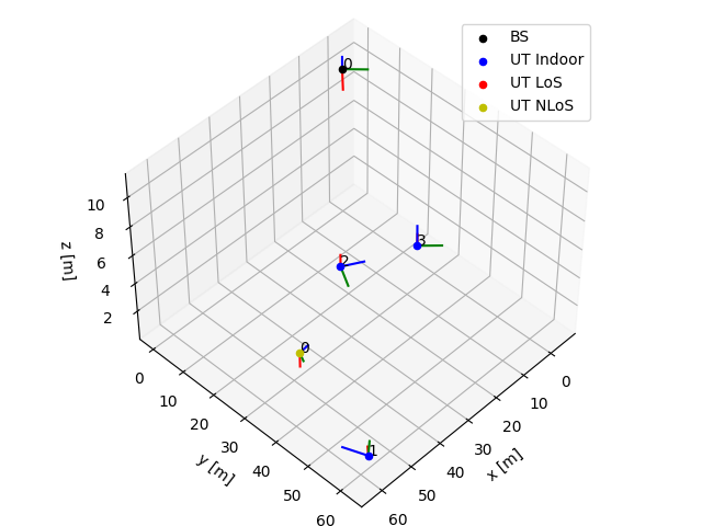
Input

• batch_size (int) – Batch size

• num_ut (int) – Number of UTs to sample per batch example

• scenario (str) – System leven model scenario. Must be one of “rma”, “umi”, or “uma”.

• min_bs_ut_dist (None or tf.float) – Minimum BS-UT distance [m]

• isd (None or tf.float) – Inter-site distance [m]

• bs_height (None or tf.float) – BS elevation [m]

• min_ut_height (None or tf.float) – Minimum UT elevation [m]

• max_ut_height (None or tf.float) – Maximum UT elevation [m]

• indoor_probability (None or tf.float) – Probability of a UT to be indoor

• min_ut_velocity (None or tf.float) – Minimum UT velocity [m/s]

• max_ut_velocity (None or tf.float) – Maximim UT velocity [m/s]

• dtype (tf.DType) – Datatype to use for internal processing and output. If a complex datatype is provided, the corresponding precision of real components is used. Defaults to tf.complex64 (tf.float32).

Output

• ut_loc ([batch_size, num_ut, 3], tf.float) – UTs locations

• bs_loc ([batch_size, 1, 3], tf.float) – BS location. Set to (0,0,0) for all batch examples.

• ut_orientations ([batch_size, num_ut, 3], tf.float) – UTs orientations [radian]

• bs_orientations ([batch_size, 1, 3], tf.float) – BS orientations [radian]. Oriented towards the center of the sector.

• ut_velocities ([batch_size, num_ut, 3], tf.float) – UTs velocities [m/s]

• in_state ([batch_size, num_ut], tf.float) – Indoor/outdoor state of UTs. True means indoor, False means outdoor.

gen_single_sector_topology_interferers

sionna.channel.gen_single_sector_topology_interferers(batch_size, num_ut, num_interferer, scenario, min_bs_ut_dist=None, isd=None, bs_height=None, min_ut_height=None, max_ut_height=None, indoor_probability=None, min_ut_velocity=None, max_ut_velocity=None, dtype=tf.complex64)

Generate a batch of topologies consisting of a single BS located at the origin, num_ut UTs randomly and uniformly dropped in a cell sector, and num_interferer interfering UTs randomly dropped in the adjacent cells.

The following picture shows how UTs are sampled

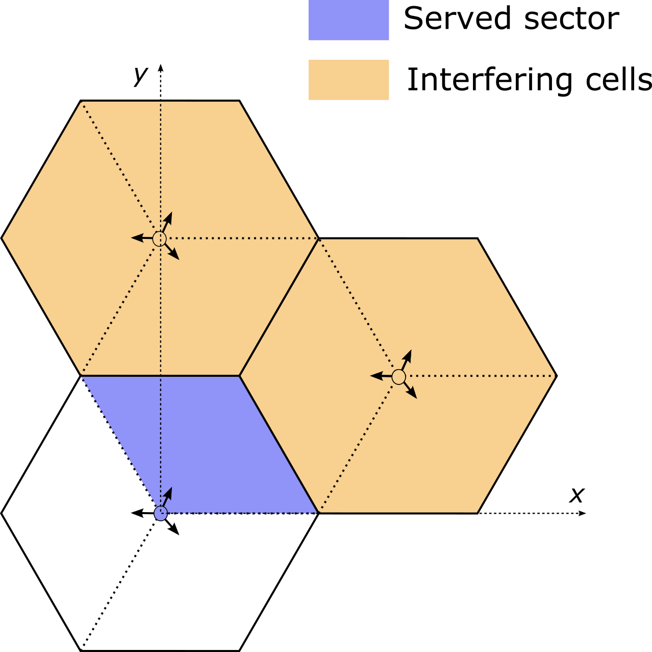
UTs orientations are randomly and uniformly set, whereas the BS orientation is set such that it is oriented towards the center of the sector it serves.

The drop configuration can be controlled through the optional parameters. Parameters set to None are set to valid values according to the chosen scenario (see [TR38901]).

The returned batch of topologies can be used as-is with the set_topology() method of the system level models, i.e. UMi, UMa, and RMa.

In the returned ut_loc, ut_orientations, ut_velocities, and in_state tensors, the first num_ut items along the axis with index 1 correspond to the served UTs, whereas the remaining num_interferer items correspond to the interfering UTs.

Example

>>> # Create antenna arrays
>>> bs_array = PanelArray(num_rows_per_panel = 4,
...                      num_cols_per_panel = 4,
...                      polarization = 'dual',
...                      polarization_type = 'VH',
...                      antenna_pattern = '38.901',
...                      carrier_frequency = 3.5e9)
>>>
>>> ut_array = PanelArray(num_rows_per_panel = 1,
...                       num_cols_per_panel = 1,
...                       polarization = 'single',
...                       polarization_type = 'V',
...                       antenna_pattern = 'omni',
...                       carrier_frequency = 3.5e9)
>>> # Create channel model
>>> channel_model = UMi(carrier_frequency = 3.5e9,
...                     o2i_model = 'low',
...                     ut_array = ut_array,
...                     bs_array = bs_array,
...                     direction = 'uplink')
>>> # Generate the topology
>>> topology = gen_single_sector_topology_interferers(batch_size = 100,
...                                                   num_ut = 4,
...                                                   num_interferer = 4,
...                                                   scenario = 'umi')
>>> # Set the topology
>>> ut_loc, bs_loc, ut_orientations, bs_orientations, ut_velocities, in_state = topology
>>> channel_model.set_topology(ut_loc,
...                            bs_loc,
...                            ut_orientations,
...                            bs_orientations,
...                            ut_velocities,
...                            in_state)
>>> channel_model.show_topology()

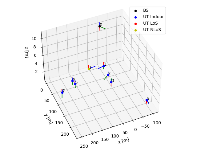
Input

• batch_size (int) – Batch size

• num_ut (int) – Number of UTs to sample per batch example

• num_interferer (int) – Number of interfeering UTs per batch example

• scenario (str) – System leven model scenario. Must be one of “rma”, “umi”, or “uma”.

• min_bs_ut_dist (None or tf.float) – Minimum BS-UT distance [m]

• isd (None or tf.float) – Inter-site distance [m]

• bs_height (None or tf.float) – BS elevation [m]

• min_ut_height (None or tf.float) – Minimum UT elevation [m]

• max_ut_height (None or tf.float) – Maximum UT elevation [m]

• indoor_probability (None or tf.float) – Probability of a UT to be indoor

• min_ut_velocity (None or tf.float) – Minimum UT velocity [m/s]

• max_ut_velocity (None or tf.float) – Maximim UT velocity [m/s]

• dtype (tf.DType) – Datatype to use for internal processing and output. If a complex datatype is provided, the corresponding precision of real components is used. Defaults to tf.complex64 (tf.float32).

Output

• ut_loc ([batch_size, num_ut, 3], tf.float) – UTs locations. The first num_ut items along the axis with index 1 correspond to the served UTs, whereas the remaining num_interferer items correspond to the interfeering UTs.

• bs_loc ([batch_size, 1, 3], tf.float) – BS location. Set to (0,0,0) for all batch examples.

• ut_orientations ([batch_size, num_ut, 3], tf.float) – UTs orientations [radian]. The first num_ut items along the axis with index 1 correspond to the served UTs, whereas the remaining num_interferer items correspond to the interfeering UTs.

• bs_orientations ([batch_size, 1, 3], tf.float) – BS orientation [radian]. Oriented towards the center of the sector.

• ut_velocities ([batch_size, num_ut, 3], tf.float) – UTs velocities [m/s]. The first num_ut items along the axis with index 1 correspond to the served UTs, whereas the remaining num_interferer items correspond to the interfeering UTs.

• in_state ([batch_size, num_ut], tf.float) – Indoor/outdoor state of UTs. True means indoor, False means outdoor. The first num_ut items along the axis with index 1 correspond to the served UTs, whereas the remaining num_interferer items correspond to the interfeering UTs.

exp_corr_mat

sionna.channel.exp_corr_mat(a, n, dtype=tf.complex64)

Generate exponential correlation matrices.

This function computes for every element \(a\) of a complex-valued tensor \(\mathbf{a}\) the corresponding \(n\times n\) exponential correlation matrix \(\mathbf{R}(a,n)\), defined as (Eq. 1, [MAL2018]):

\[\begin{split}\mathbf{R}(a,n)_{i,j} = \begin{cases} 1 & \text{if } i=j\\ a^{i-j} & \text{if } i>j\\ (a^\star)^{j-i} & \text{if } j<i, j=1,\dots,n\\ \end{cases}\end{split}\]

where \(|a|<1\) and \(\mathbf{R}\in\mathbb{C}^{n\times n}\).

Input

• a ([n_0, …, n_k], tf.complex) – A tensor of arbitrary rank whose elements have an absolute value smaller than one.

• n (int) – Number of dimensions of the output correlation matrices.

• dtype (tf.complex64, tf.complex128) – The dtype of the output.

Output

R ([n_0, …, n_k, n, n], tf.complex) – A tensor of the same dtype as the input tensor \(\mathbf{a}\).

one_ring_corr_mat

sionna.channel.one_ring_corr_mat(phi_deg, num_ant, d_h=0.5, sigma_phi_deg=15, dtype=tf.complex64)

Generate covariance matrices from the one-ring model.

This function generates approximate covariance matrices for the so-called one-ring model (Eq. 2.24) [BHS2017]. A uniform linear array (ULA) with uniform antenna spacing is assumed. The elements of the covariance matrices are computed as:

\[\mathbf{R}_{\ell,m} = \exp\left( j2\pi d_\text{H} (\ell -m)\sin(\varphi) \right) \exp\left( -\frac{\sigma_\varphi^2}{2} \left( 2\pi d_\text{H}(\ell -m)\cos(\varphi) \right)^2 \right)\]

for \(\ell,m = 1,\dots, M\), where \(M\) is the number of antennas, \(\varphi\) is the angle of arrival, \(d_\text{H}\) is the antenna spacing in multiples of the wavelength, and \(\sigma^2_\varphi\) is the angular standard deviation.

Input

• phi_deg ([n_0, …, n_k], tf.float) – A tensor of arbitrary rank containing azimuth angles (deg) of arrival.

• num_ant (int) – Number of antennas

• d_h (float) – Antenna spacing in multiples of the wavelength. Defaults to 0.5.

• sigma_phi_deg (float) – Angular standard deviation (deg). Defaults to 15 (deg). Values greater than 15 should not be used as the approximation becomes invalid.

• dtype (tf.complex64, tf.complex128) – The dtype of the output.

Output

R ([n_0, …, n_k, num_ant, nun_ant], dtype) – Tensor containing the covariance matrices of the desired dtype.

References:

TR38901(1,2,3,4,5,6,7,8,9,10,11,12,13,14,15,16,17,18,19,20,21)

3GPP TR 38.901, “Study on channel model for frequencies from 0.5 to 100 GHz”, Release 16.1

TS38141-1

3GPP TS 38.141-1 “Base Station (BS) conformance testing Part 1: Conducted conformance testing”, Release 17

Tse

D. Tse and P. Viswanath, “Fundamentals of wireless communication“, Cambridge university press, 2005.

SoS

3. Xiao, Y. R. Zheng and N. C. Beaulieu, “Novel Sum-of-Sinusoids Simulation Models for Rayleigh and Rician Fading Channels,” in IEEE Transactions on Wireless Communications, vol. 5, no. 12, pp. 3667-3679, December 2006, doi: 10.1109/TWC.2006.256990.

MAL2018

Ranjan K. Mallik, “The exponential correlation matrix: Eigen-analysis and applications”, IEEE Trans. Wireless Commun., vol. 17, no. 7, pp. 4690-4705, Jul. 2018.

BHS2017

Emil Björnson, Jakob Hoydis and Luca Sanguinetti (2017), “Massive MIMO Networks: Spectral, Energy, and Hardware Efficiency”, Foundations and Trends in Signal Processing: Vol. 11, No. 3-4, pp 154–655.