Utility Functions

This module provides utility functions for the FEC package. It also provides serval functions to simplify EXIT analysis of iterative receivers.

(Binary) Linear Codes

Several functions are provided to convert parity-check matrices into generator matrices and vice versa. Please note that currently only binary codes are supported.

# load example parity-check matrix
pcm, k, n, coderate = load_parity_check_examples(pcm_id=3)

Note that many research projects provide their parity-check matrices in the alist format [MacKay] (e.g., see [UniKL]). The follwing code snippet provides an example of how to import an external LDPC parity-check matrix from an alist file and how to set-up an encoder/decoder.

# load external example parity-check matrix in alist format
al = load_alist(path=filename)
pcm, k, n, coderate = alist2mat(al)

# the linear encoder can be directly initialized with a parity-check matrix
encoder = LinearEncoder(pcm, is_pcm=True)

# initalize BP decoder for the given parity-check matrix
decoder = LDPCBPDecoder(pcm, num_iter=20)

# and run simulation with random information bits
no = 1.
batch_size = 10
num_bits_per_symbol = 2

source = BinarySource()
mapper = Mapper("qam", num_bits_per_symbol)
channel = AWGN()
demapper = Demapper("app", "qam", num_bits_per_symbol)

u = source([batch_size, k])
c = encoder(u)
x = mapper(c)
y = channel(x, no)
llr = demapper(y, no)
c_hat = decoder(llr)

sionna.phy.fec.utils.load_parity_check_examples(pcm_id, verbose=False)

Loads parity-check matrices of built-in example codes.

This utility function loads predefined example codes, including Hamming, BCH, and LDPC codes. The following codes are available:

• pcm_id =0 : (7,4) Hamming code with k=4 information bits and n=7 codeword length.

• pcm_id =1 : (63,45) BCH code with k=45 information bits and n=63 codeword length.

• pcm_id =2 : (127,106) BCH code with k=106 information bits and n=127 codeword length.

• pcm_id =3 : Random LDPC code with variable node degree 3 and check node degree 6, with k=50 information bits and n=100 codeword length.

• pcm_id =4 : 802.11n LDPC code with k=324 information bits and n=648 codeword length.

Parameters:

• pcm_id (int) – An integer identifying the code matrix to load.

• verbose (bool, (default False)) – If True, prints the code parameters.

Returns:

• pcm (numpy.ndarray) – Array containing the parity-check matrix (values are 0 and 1).

• k (int) – Number of information bits.

• n (int) – Number of codeword bits.

• coderate (float) – Code rate, assuming full rank of the parity-check matrix.

sionna.phy.fec.utils.alist2mat(alist, verbose=True)

Converts an alist [MacKay] code definition to a NumPy parity-check matrix.

This function converts an alist format representation of a code’s parity-check matrix to a NumPy array. Many example codes in alist format can be found in [UniKL].

About the alist format (see [MacKay] for details):

• Row 1: Defines the parity-check matrix dimensions m x n.

• Row 2: Contains two integers, max_CN_degree and max_VN_degree.

• Row 3: Lists the degrees of all n variable nodes (columns).

• Row 4: Lists the degrees of all m check nodes (rows).

• Next n rows: Non-zero entries of each column, zero-padded as needed.

• Following m rows: Non-zero entries of each row, zero-padded as needed.

Parameters:

• alist (list) – Nested list in alist format [MacKay] representing the parity-check matrix.

• verbose (bool, (default True)) – If True, prints the code parameters.

Returns:

• pcm (numpy.ndarray) – NumPy array of shape [n - k, n] representing the parity-check matrix.

• k (int) – Number of information bits.

• n (int) – Number of codeword bits.

• coderate (float) – Code rate of the code.

Notes

Use load_alist to import an alist from a text file.

Example

The following code snippet imports an alist from a file called filename:

al = load_alist(path=filename)
pcm, k, n, coderate = alist2mat(al)

sionna.phy.fec.utils.load_alist(path)

Reads an alist file and returns a nested list describing a code’s parity-check matrix.

This function reads a file in alist format [MacKay] and returns a nested list representing the parity-check matrix. Numerous example codes in alist format are available in [UniKL].

Parameters:

path (str) – Path to the alist file to be loaded.

Returns:

A nested list containing the imported alist data representing the parity-check matrix.

Return type:

list

sionna.phy.fec.utils.generate_reg_ldpc(v, c, n, allow_flex_len=True, verbose=True)

Generates a random regular (v, c) LDPC code.

This function generates a random Low-Density Parity-Check (LDPC) parity-check matrix of length n where each variable node (VN) has degree v and each check node (CN) has degree c. Note that the generated LDPC code is not optimized to avoid short cycles, which may result in a non-negligible error floor. For encoding, the LinearEncoder block can be used, but the construction does not guarantee that the parity-check matrix (pcm) has full rank.

Parameters:

• v (int) – Desired degree of each variable node (VN).

• c (int) – Desired degree of each check node (CN).

• n (int) – Desired codeword length.

• allow_flex_len (bool, (default True)) – If True, the resulting codeword length may be slightly increased to meet the degree requirements.

• verbose (bool, (default True)) – If True, prints code parameters.

Returns:

• pcm (numpy.ndarray) – Parity-check matrix of shape [n - k, n].

• k (int) – Number of information bits per codeword.

• n (int) – Number of codeword bits.

• coderate (float) – Code rate of the LDPC code.

Notes

This algorithm is designed only for regular node degrees. To achieve state-of-the-art bit-error-rate performance, optimizing irregular degree profiles is usually necessary (see [tenBrink]).

sionna.phy.fec.utils.make_systematic(mat, is_pcm=False)

Converts a binary matrix to its systematic form.

This function transforms a binary matrix into systematic form, where the first k columns (or last k columns if is_pcm is True) form an identity matrix.

Parameters:

• mat (numpy.ndarray) – Binary matrix of shape [k, n] to be transformed to systematic form.

• is_pcm (bool, (default False)) – If True, mat is treated as a parity-check matrix, and the identity part will be placed in the last k columns.

Returns:

• mat_sys (numpy.ndarray) – Binary matrix in systematic form, where the first k columns (or last k columns if is_pcm is True) form the identity matrix.

• column_swaps (list of tuple of int) – A list of integer tuples representing the column swaps performed to achieve the systematic form, in order of execution.

Notes

This function may swap columns of the input matrix to achieve systematic form. As a result, the output matrix represents a permuted version of the code, defined by the column_swaps list. To revert to the original column order, apply the inverse permutation in reverse order of the swaps.

If is_pcm is True, indicating a parity-check matrix, the identity matrix portion will be arranged in the last k columns.

sionna.phy.fec.utils.gm2pcm(gm, verify_results=True)

Generates the parity-check matrix for a given generator matrix.

This function converts the generator matrix gm (denoted as $\mathbf{G}$) to systematic form and uses the following relationship to compute the parity-check matrix $\mathbf{H}$ over GF(2):

$$\begin{array}{}\text{(1)}& \mathbf{G}=[\mathbf{I}|\mathbf{M}]\Rightarrow \mathbf{H}=[{\mathbf{M}}^T|\mathbf{I}].\end{array}$$

This is derived from the requirement for an all-zero syndrome, such that:

$$\mathbf{H}{\mathbf{c}}^T=\mathbf{H}\ast (\mathbf{u}\ast \mathbf{G}{)}^T=\mathbf{H}\ast {\mathbf{G}}^T\ast {\mathbf{u}}^T=\mathbf{0},$$

where $\mathbf{c}$ represents an arbitrary codeword and $\mathbf{u}$ the corresponding information bits.

This leads to:

$$\begin{array}{}\text{(2)}& \mathbf{G}\ast {\mathbf{H}}^T=\mathbf{0}.\end{array}$$

It can be seen that (1) satisfies (2), as in GF(2):

$$[\mathbf{I}|\mathbf{M}]\ast [{\mathbf{M}}^T|\mathbf{I}{]}^T=\mathbf{M}+\mathbf{M}=\mathbf{0}.$$

Parameters:

• gm (numpy.ndarray) – Binary generator matrix of shape [k, n].

• verify_results (bool, (default True)) – If True, verifies that the generated parity-check matrix is orthogonal to the generator matrix in GF(2).

Returns:

Binary parity-check matrix of shape [n - k, n].

Return type:

numpy.ndarray

Notes

This function requires gm to have full rank. An error is raised if gm does not meet this requirement.

sionna.phy.fec.utils.pcm2gm(pcm, verify_results=True)

Generates the generator matrix for a given parity-check matrix.

This function converts the parity-check matrix pcm (denoted as $\mathbf{H}$) to systematic form and uses the following relationship to compute the generator matrix $\mathbf{G}$ over GF(2):

$$\begin{array}{}\text{(1)}& \mathbf{G}=[\mathbf{I}|\mathbf{M}]\Rightarrow \mathbf{H}=[{\mathbf{M}}^T|\mathbf{I}].\end{array}$$

This derivation is based on the requirement for an all-zero syndrome:

$$\mathbf{H}{\mathbf{c}}^T=\mathbf{H}\ast (\mathbf{u}\ast \mathbf{G}{)}^T=\mathbf{H}\ast {\mathbf{G}}^T\ast {\mathbf{u}}^T=\mathbf{0},$$

where $\mathbf{c}$ represents an arbitrary codeword and $\mathbf{u}$ the corresponding information bits.

This leads to:

$$\begin{array}{}\text{(2)}& \mathbf{G}\ast {\mathbf{H}}^T=\mathbf{0}.\end{array}$$

It can be shown that (1) satisfies (2), as in GF(2):

$$[\mathbf{I}|\mathbf{M}]\ast [{\mathbf{M}}^T|\mathbf{I}{]}^T=\mathbf{M}+\mathbf{M}=\mathbf{0}.$$

Parameters:

• pcm (numpy.ndarray) – Binary parity-check matrix of shape [n - k, n].

• verify_results (bool, (default True)) – If True, verifies that the generated generator matrix is orthogonal to the parity-check matrix in GF(2).

Returns:

Binary generator matrix of shape [k, n].

Return type:

numpy.ndarray

Notes

This function requires pcm to have full rank. An error is raised if pcm does not meet this requirement.

sionna.phy.fec.utils.verify_gm_pcm(gm, pcm)

Verifies that the generator matrix $\mathbf{G}$ (gm) and parity-check matrix $\mathbf{H}$ (pcm) are orthogonal in GF(2).

For a valid code with an all-zero syndrome, the following condition must hold:

$$\mathbf{H}{\mathbf{c}}^T=\mathbf{H}\ast (\mathbf{u}\ast \mathbf{G}{)}^T=\mathbf{H}\ast {\mathbf{G}}^T\ast {\mathbf{u}}^T=\mathbf{0},$$

where $\mathbf{c}$ represents an arbitrary codeword and $\mathbf{u}$ the corresponding information bits.

Since $\mathbf{u}$ can be arbitrary, this leads to the condition:

$$\mathbf{H}\ast {\mathbf{G}}^T=\mathbf{0}.$$

Parameters:

• gm (numpy.ndarray) – Binary generator matrix of shape [k, n].

• pcm (numpy.ndarray) – Binary parity-check matrix of shape [n - k, n].

Returns:

True if gm and pcm define a valid pair of orthogonal parity-check and generator matrices in GF(2).

Return type:

bool

EXIT Analysis

The LDPC BP decoder allows to track the internal information flow (extrinsic information) during decoding via callbacks. This can be plotted in so-called EXIT Charts [tenBrinkEXIT] to visualize the decoding convergence.

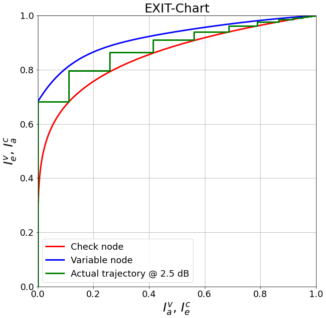
This short code snippet shows how to generate and plot EXIT charts:

# parameters
ebno_db = 2.5 # simulation SNR
batch_size = 10000
num_bits_per_symbol = 2 # QPSK
num_iter = 20 # number of decoding iterations

pcm_id = 4 # decide which parity check matrix should be used (0-2: BCH; 3: (3,6)-LDPC 4: LDPC 802.11n
pcm, k, n , coderate = load_parity_check_examples(pcm_id, verbose=True)

noise_var = ebnodb2no(ebno_db=ebno_db,
                      num_bits_per_symbol=num_bits_per_symbol,
                      coderate=coderate)

# init callbacks for tracking of EXIT charts
cb_exit_vn = EXITCallback(num_iter)
cb_exit_cn = EXITCallback(num_iter)

# init components
decoder = LDPCBPDecoder(pcm,
                        hard_out=False,
                        cn_update="boxplus",
                        num_iter=num_iter,
                        v2c_callbacks=[cb_exit_vn,], # register callbacks
                        c2v_callbacks=[cb_exit_cn,],) # register callbacks

# generates fake llrs as if the all-zero codeword was transmitted over an AWNG channel with BPSK modulation
llr_source = GaussianPriorSource()


# generate fake LLRs (Gaussian approximation)
# Remark: the EXIT callbacks require all-zero codeword simulations
llr_ch = llr_source([batch_size, n], noise_var)

# simulate free running decoder (for EXIT trajectory)
decoder(llr_ch)

# calculate analytical EXIT characteristics
# Hint: these curves assume asymptotic code length, i.e., may become inaccurate in the short length regime
Ia, Iev, Iec = get_exit_analytic(pcm, ebno_db)

# and plot the analytical exit curves

plt = plot_exit_chart(Ia, Iev, Iec)

# and add simulated trajectory (requires "track_exit=True")
plot_trajectory(plt, cb_exit_vn.mi.numpy(), cb_exit_cn.mi.numpy(), ebno_db)

Remark: for rate-matched 5G LDPC codes, the EXIT approximation becomes inaccurate due to the rate-matching and the very specific structure of the code.

sionna.phy.fec.utils.plot_exit_chart(mi_a=None, mi_ev=None, mi_ec=None, title='EXIT-Chart')

Plots an EXIT-chart based on mutual information curves [tenBrinkEXIT].

This utility function generates an EXIT-chart plot. If all inputs are None, an empty EXIT chart is created; otherwise, mutual information curves are plotted.

Parameters:

• mi_a (numpy.ndarray, optional) – Array of floats representing the a priori mutual information.

• mi_v (numpy.ndarray, optional) – Array of floats representing the variable node mutual information.

• mi_c (numpy.ndarray, optional) – Array of floats representing the check node mutual information.

• title (str) – Title of the EXIT chart.

Returns:

A handle to the generated matplotlib figure.

Return type:

matplotlib.figure.Figure

sionna.phy.fec.utils.get_exit_analytic(pcm, ebno_db)

Calculates analytic EXIT curves for a given parity-check matrix.

This function extracts the degree profile from the provided parity-check matrix pcm and calculates the EXIT (Extrinsic Information Transfer) curves for variable nodes (VN) and check nodes (CN) decoders. Note that this approach relies on asymptotic analysis, which requires a sufficiently large codeword length for accurate predictions.

It assumes transmission over an AWGN channel with BPSK modulation at an SNR specified by ebno_db. For more details on the equations, see [tenBrink] and [tenBrinkEXIT].

Parameters:

• pcm (numpy.ndarray) – The parity-check matrix.

• ebno_db (float) – Channel SNR in dB.

Returns:

• mi_a (numpy.ndarray) – Array of floats containing the a priori mutual information.

• mi_ev (numpy.ndarray) – Array of floats containing the extrinsic mutual information of the variable node decoder for each mi_a value.

• mi_ec (numpy.ndarray) – Array of floats containing the extrinsic mutual information of the check node decoder for each mi_a value.

Notes

This function assumes random, unstructured parity-check matrices. Thus, applying it to parity-check matrices with specific structures or constraints may result in inaccurate EXIT predictions. Additionally, this function is based on asymptotic properties and performs best with large parity-check matrices. For more information, refer to [tenBrink].

sionna.phy.fec.utils.plot_trajectory(plot, mi_v, mi_c, ebno=None)

Plots the trajectory of an EXIT-chart.

This utility function plots the trajectory of mutual information values in an EXIT-chart, based on variable and check node mutual information values.

Parameters:

• plot (matplotlib.figure.Figure) – A handle to a matplotlib figure where the trajectory will be plotted.

• mi_v (numpy.ndarray) – Array of floats representing the variable node mutual information values.

• mi_c (numpy.ndarray) – Array of floats representing the check node mutual information values.

• ebno (float) – The Eb/No value in dB, used for the legend entry.

Miscellaneous

class sionna.phy.fec.utils.GaussianPriorSource(*, precision=None, **kwargs)

Generates synthetic Log-Likelihood Ratios (LLRs) for Gaussian channels.

Generates synthetic Log-Likelihood Ratios (LLRs) as if an all-zero codeword was transmitted over a Binary Additive White Gaussian Noise (Bi-AWGN) channel. The LLRs are generated based on either the noise variance no or mutual information. If mutual information is used, it represents the information associated with a binary random variable observed through an AWGN channel.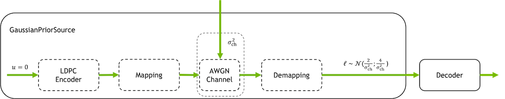

The generated LLRs follow a Gaussian distribution with parameters:

$${\sigma }_{\text{llr}}^2=\frac{4}{{\sigma }_{\text{ch}}^2}$$

$${\mu }_{\text{llr}}=\frac{{\sigma }_{\text{llr}}^2}{2}$$

where ${\sigma }_{\text{ch}}^2$ is the noise variance specified by no.

If the mutual information is provided as input, the J-function as described in [Brannstrom] is used to relate the mutual information to the corresponding LLR distribution.

Parameters:

precision (None (default) | ‘single’ | ‘double’) – Precision used for internal calculations and outputs. If set to None, precision is used.

Input:

• output_shape (tf.int) – Integer tensor or Python list defining the shape of the generated LLR tensor.

• no (None (default) | tf.float) – Scalar defining the noise variance for the synthetic AWGN channel.

• mi (None (default) | tf.float) – Scalar defining the mutual information for the synthetic AWGN channel. Only used of no is None.

Output:

tf.Tensor of dtype ``dtype`` (defaults to `tf.float32`) – Tensor with shape defined by output_shape.

sionna.phy.fec.utils.bin2int(arr)

Converts a binary array to its integer representation.

This function converts an iterable binary array to its equivalent integer. For example, [1, 0, 1] is converted to 5.

Parameters:

arr (iterable of int or float) – An iterable that contains binary values (0’s and 1’s).

Returns:

The integer representation of the binary array.

Return type:

int

sionna.phy.fec.utils.int2bin(num, length)

Converts an integer to a binary list of specified length.

This function converts an integer num to a list of 0’s and 1’s, with the binary representation padded to a length of length. Both num and length must be non-negative.

For example:

• If num = 5 and length = 4, the output is [0, 1, 0, 1].

• If num = 12 and length = 3, the output is [1, 0, 0] (truncated to length).

Parameters:

• num (int) – The integer to be converted into binary representation.

• length (int) – The desired length of the binary output list.

Returns:

A list of 0’s and 1’s representing the binary form of num, padded or truncated to a length of length.

Return type:

list of int

sionna.phy.fec.utils.bin2int_tf(arr)

Converts a binary tensor to an integer tensor.

Interprets the binary representation across the last dimension of arr, from most significant to least significant bit. For example, an input of [0, 1, 1] is converted to 3.

Parameters:

arr (tf.Tensor) – Tensor of integers or floats containing binary values (0’s and 1’s) along the last dimension.

Returns:

Tensor with the integer representation of arr.

Return type:

tf.Tensor

sionna.phy.fec.utils.int2bin_tf(ints, length)

Converts an integer tensor to a binary tensor with specified bit length.

This function converts each integer in the input tensor ints to a binary representation, with an additional dimension of size length added at the end to represent the binary bits. The length parameter must be non-negative.

Parameters:

• ints (tf.Tensor) – Tensor of arbitrary shape […, k] containing integers to be converted into binary representation.

• length (int) – An integer specifying the bit length of the binary representation for each integer.

Returns:

A tensor of the same shape as ints with an additional dimension of size length at the end, i.e., shape […, k, length]. This tensor contains the binary representation of each integer in ints.

Return type:

tf.Tensor

sionna.phy.fec.utils.int_mod_2(x)

Modulo 2 operation and implicit rounding for floating point inputs

Performs more efficient modulo-2 operation for integer inputs. Uses tf.math.floormod for floating inputs and applies implicit rounding for floating point inputs.

Parameters:

x (tf.Tensor) – Tensor to which the modulo 2 operation is applied.

Returns:

x_mod – Binary Tensor containing the result of the modulo 2 operation, with the same shape as x.

Return type:

tf.Tensor

sionna.phy.fec.utils.llr2mi(llr, s=None, reduce_dims=True)

Approximates the mutual information based on Log-Likelihood Ratios (LLRs).

This function approximates the mutual information for a given set of llr values, assuming an all-zero codeword transmission as derived in [Hagenauer]:

$$I\approx 1-\sum {\log }_2(1+{\mathrm{e}}^{-\text{llr}})$$

The approximation relies on the symmetry condition:

$$p(\text{llr}|x=0)=p(\text{llr}|x=1)\cdot \exp (\text{llr})$$

For cases where the transmitted codeword is not all-zero, this method requires knowledge of the original bit sequence s to adjust the LLR signs accordingly, simulating an all-zero codeword transmission.

Note that the LLRs are defined as $\frac{p(x=1)}{p(x=0)}$, which reverses the sign compared to the solution in [Hagenauer].

Parameters:

• llr (tf.float) – Tensor of arbitrary shape containing LLR values.

• s (None | tf.float) – Tensor of the same shape as llr representing the signs of the transmitted sequence (assuming BPSK), with values of +/-1.

• reduce_dims (bool, (default True)) – If True, reduces all dimensions and returns a scalar. If False, averages only over the last dimension.

Returns:

mi – If reduce_dims is True, returns a scalar tensor. Otherwise, returns a tensor with the same shape as llr except for the last dimension, which is removed. Contains the approximated mutual information.

Return type:

tf.float

sionna.phy.fec.utils.j_fun(mu)

Computes the J-function

The J-function relates mutual information to the mean of Gaussian-distributed Log-Likelihood Ratios (LLRs) using the Gaussian approximation. This function implements the approximation proposed in [Brannstrom]:

$$J(\mu )\approx {(1-2^{H_{\text{1}}(2\mu {)}^{H_{\text{2}}}})}^{H_{\text{3}}}$$

where $\mu$ represents the mean of the LLR distribution, and the constants are defined as $H_{\text{1}}=0.3073$, $H_{\text{2}}=0.8935$, and $H_{\text{3}}=1.1064$.

Input values are clipped to [1e-10, 1000] for numerical stability. The output is clipped to a maximum LLR of 20.

Parameters:

mu (tf.float32) – Tensor of arbitrary shape, representing the mean of the LLR values.

Returns:

Tensor of the same shape and dtype as mu, containing the calculated mutual information values.

Return type:

tf.float32

sionna.phy.fec.utils.j_fun_inv(mi)

Computes the inverse of the J-function

The J-function relates mutual information to the mean of Gaussian-distributed Log-Likelihood Ratios (LLRs) using the Gaussian approximation. This function computes the inverse J-function based on the approximation proposed in [Brannstrom]:

$$J(\mu )\approx {(1-2^{H_{\text{1}}(2\mu {)}^{H_{\text{2}}}})}^{H_{\text{3}}}$$

where $\mu$ is the mean of the LLR distribution, and constants are defined as $H_{\text{1}}=0.3073$, $H_{\text{2}}=0.8935$, and $H_{\text{3}}=1.1064$.

Input values are clipped to [1e-10, 1] for numerical stability. The output is clipped to a maximum LLR of 20.

Parameters:

mi (tf.float32) – Tensor of arbitrary shape, representing mutual information values.

Returns:

Tensor of the same shape and dtype as mi, containing the computed mean values of the LLR distribution.

Return type:

tf.float32

References:

[tenBrinkEXIT] (1,2,3)

S. ten Brink, “Convergence Behavior of Iteratively Decoded Parallel Concatenated Codes,” IEEE Transactions on Communications, vol. 49, no. 10, pp. 1727-1737, 2001.

[Brannstrom] (1,2,3)

F. Brannstrom, L. K. Rasmussen, and A. J. Grant, “Convergence analysis and optimal scheduling for multiple concatenated codes,” IEEE Trans. Inform. Theory, vol. 51, no. 9, pp. 3354–3364, 2005.

[Hagenauer] (1,2)

J. Hagenauer, “The Turbo Principle in Mobile Communications,” in Proc. IEEE Int. Symp. Inf. Theory and its Appl. (ISITA), 2002.

[tenBrink] (1,2,3)

S. ten Brink, G. Kramer, and A. Ashikhmin, “Design of low-density parity-check codes for modulation and detection,” IEEE Trans. Commun., vol. 52, no. 4, pp. 670–678, Apr. 2004.

[MacKay] (1,2,3,4,5)

http://www.inference.org.uk/mackay/codes/alist.html

[UniKL] (1,2,3)

https://www.uni-kl.de/en/channel-codes/