Signal

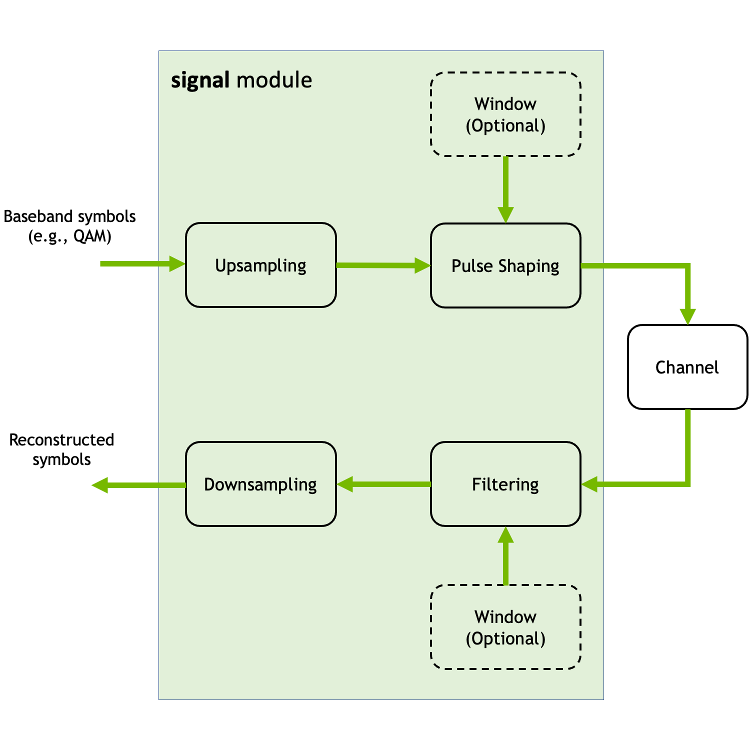
This module contains classes and functions for filtering (pulse shaping), windowing, and up- and downsampling. The following figure shows the different components that can be implemented using this module.

This module also contains utility functions for computing the (inverse) discrete Fourier transform (FFT/IFFT), and for empirically computing the power spectral density (PSD) and adjacent channel leakage ratio (ACLR) of a signal.

The following code snippet shows how to filter a sequence of QAM baseband symbols using a root-raised-cosine filter with a Hann window:

# Create batch of QAM-16 sequences
batch_size = 128
num_symbols = 1000
num_bits_per_symbol = 4
x = QAMSource(num_bits_per_symbol)([batch_size, num_symbols])

# Create a root-raised-cosine filter with Hann windowing
beta = 0.22 # Roll-off factor
span_in_symbols = 32 # Filter span in symbols
samples_per_symbol = 4 # Number of samples per symbol, i.e., the oversampling factor
rrcf_hann = RootRaisedCosineFilter(span_in_symbols, samples_per_symbol, beta, window="hann")

# Create instance of the Upsampling layer
us = Upsampling(samples_per_symbol)

# Upsample the baseband x
x_us = us(x)

# Filter the upsampled sequence
x_rrcf = rrcf_hann(x_us)

On the receiver side, one would recover the baseband symbols as follows:

# Instantiate a downsampling layer
ds = Downsampling(samples_per_symbol, rrcf_hann.length-1, num_symbols)

# Apply the matched filter
x_mf = rrcf_hann(x_rrcf)

# Recover the transmitted symbol sequence
x_hat = ds(x_mf)

Filters

class sionna.phy.signal.SincFilter(span_in_symbols, samples_per_symbol, window=None, normalize=True, precision=None, **kwargs)

Block for applying a sinc filter of length K to an input x of length N

The sinc filter is defined by

$$h(t)=\frac{1}{T}\text{sinc}\left(\frac{t}{T}\right)$$

where $T$ the symbol duration.

The filter length K is equal to the filter span in symbols (span_in_symbols) multiplied by the oversampling factor (samples_per_symbol). If this product is even, a value of one will be added.

The filter is applied through discrete convolution.

An optional windowing function window can be applied to the filter.

The dtype of the output is tf.float if both x and the filter coefficients have dtype tf.float. Otherwise, the dtype of the output is tf.complex.

Three padding modes are available for applying the filter:

• “full” (default): Returns the convolution at each point of overlap between x and the filter. The length of the output is N + K - 1. Zero-padding of the input x is performed to compute the convolution at the borders.

• “same”: Returns an output of the same length as the input x. The convolution is computed such that the coefficients of the input x are centered on the coefficient of the filter with index (K-1)/2. Zero-padding of the input signal is performed to compute the convolution at the borders.

• “valid”: Returns the convolution only at points where x and the filter completely overlap. The length of the output is N - K + 1.

Parameters:

• span_in_symbols (int) – Filter span as measured by the number of symbols

• samples_per_symbol (int) – Number of samples per symbol, i.e., the oversampling factor

• window (None (default) | Window | “hann” | “hamming” | “blackman”) – Window that is applied to the filter coefficients

• normalize (bool, (default True)) – If True, the filter is normalized to have unit power

• precision (None (default) | “single” | “double”) – Precision used for internal calculations and outputs. If set to None, precision is used.

Input:

• x ([…,N], tf.complex or tf.float) – Input to which the filter is applied along the last dimension

• padding (“full” (default) | “valid” | “same”) – Padding mode for convolving x and the filter

• conjugate (bool, (default False)) – If True, the complex conjugate of the filter is applied.

Output:

y ([…,M], tf.complex or tf.float) – Filtered input. The length M depends on the padding.

property aclr

ACLR of the filter

This ACLR corresponds to what one would obtain from using this filter as pulse shaping filter on an i.i.d. sequence of symbols. The in-band is assumed to range from [-0.5, 0.5] in normalized frequency.

tf.float : ACLR in linear scale

property coefficients

Set/get raw filter coefficients

Type:

[K], tf.float of tf.complex

property length

Filter length in samples

Type:

int

property normalize

If True the filter is normalized to have unit power.

Type:

bool

property sampling_times

Sampling times in multiples of the symbol duration

Type:

[K], numpy.float32

show(response='impulse', scale='lin')

Plot the impulse or magnitude response

Plots the impulse response (time domain) or magnitude response (frequency domain) of the filter.

For the computation of the magnitude response, a minimum DFT size of 1024 is assumed which is obtained through zero padding of the filter coefficients in the time domain.

Input:

• response (“impulse” (default) | “magnitude”) – Desired response type

• scale (“lin” (default) | “db”) – y-scale of the magnitude response. Can be “lin” (i.e., linear) or “db” (, i.e., Decibel).

property window

Get/set window function that is applied to the filter coefficients

Type:

Window

class sionna.phy.signal.RaisedCosineFilter(span_in_symbols, samples_per_symbol, beta, window=None, normalize=True, precision=None, **kwargs)

Block for applying a raised-cosine filter of length K to an input x of length N

The raised-cosine filter is defined by

$$\begin{array}{r}h(t)=\{\begin{array}{ll}\frac{\pi }{4T}\text{sinc}\left(\frac{1}{2\beta }\right),& \text{ if }t=\pm \frac{T}{2\beta }\\ \frac{1}{T}\text{sinc}\left(\frac{t}{T}\right)\frac{\cos \left(\frac{\pi \beta t}{T}\right)}{1-{\left(\frac{2\beta t}{T}\right)}^2},& \text{otherwise}\end{array}\end{array}$$

where $\beta$ is the roll-off factor and $T$ the symbol duration.

The filter length K is equal to the filter span in symbols (span_in_symbols) multiplied by the oversampling factor (samples_per_symbol). If this product is even, a value of one will be added.

The filter is applied through discrete convolution.

An optional windowing function window can be applied to the filter.

The dtype of the output is tf.float if both x and the filter coefficients have dtype tf.float. Otherwise, the dtype of the output is tf.complex.

Three padding modes are available for applying the filter:

• “full” (default): Returns the convolution at each point of overlap between x and the filter. The length of the output is N + K - 1. Zero-padding of the input x is performed to compute the convolution at the borders.

• “same”: Returns an output of the same length as the input x. The convolution is computed such that the coefficients of the input x are centered on the coefficient of the filter with index (K-1)/2. Zero-padding of the input signal is performed to compute the convolution at the borders.

• “valid”: Returns the convolution only at points where x and the filter completely overlap. The length of the output is N - K + 1.

Parameters:

• span_in_symbols (int) – Filter span as measured by the number of symbols

• samples_per_symbol (int) – Number of samples per symbol, i.e., the oversampling factor

• beta (float) – Roll-off factor. Must be in the range $[0,1]$.

• window (None (default) | Window | “hann” | “hamming” | “blackman”) – Window that is applied to the filter coefficients

• normalize (bool, (default True)) – If True, the filter is normalized to have unit power.

• precision (None (default) | “single” | “double”) – Precision used for internal calculations and outputs. If set to None, precision is used.

Input:

• x ([…,N], tf.complex or tf.float) – Input to which the filter is applied along the last dimension

• padding (“full” (default) | “valid” | “same”) – Padding mode for convolving x and the filter

• conjugate (bool, (default False)) – If True, the complex conjugate of the filter is applied.

Output:

y ([…,M], tf.complex or tf.float) – Filtered input. The length M depends on the padding.

property aclr

ACLR of the filter

This ACLR corresponds to what one would obtain from using this filter as pulse shaping filter on an i.i.d. sequence of symbols. The in-band is assumed to range from [-0.5, 0.5] in normalized frequency.

tf.float : ACLR in linear scale

property beta

Roll-off factor

Type:

float

property coefficients

Set/get raw filter coefficients

Type:

[K], tf.float of tf.complex

property length

Filter length in samples

Type:

int

property normalize

If True the filter is normalized to have unit power.

Type:

bool

property sampling_times

Sampling times in multiples of the symbol duration

Type:

[K], numpy.float32

show(response='impulse', scale='lin')

Plot the impulse or magnitude response

Plots the impulse response (time domain) or magnitude response (frequency domain) of the filter.

For the computation of the magnitude response, a minimum DFT size of 1024 is assumed which is obtained through zero padding of the filter coefficients in the time domain.

Input:

• response (“impulse” (default) | “magnitude”) – Desired response type

• scale (“lin” (default) | “db”) – y-scale of the magnitude response. Can be “lin” (i.e., linear) or “db” (, i.e., Decibel).

property window

Get/set window function that is applied to the filter coefficients

Type:

Window

class sionna.phy.signal.RootRaisedCosineFilter(span_in_symbols, samples_per_symbol, beta, window=None, normalize=True, precision=None, **kwargs)

Block for applying a root-raised-cosine filter of length K to an input x of length N

The root-raised-cosine filter is defined by

$$\begin{array}{r}h(t)=\{\begin{array}{ll}\frac{1}{T}(1+\beta (\frac{4}{\pi }-1)),& \text{ if }t=0\\ \frac{\beta }{T\sqrt{2}}[(1+\frac{2}{\pi })\sin \left(\frac{\pi }{4\beta }\right)+(1-\frac{2}{\pi })\cos \left(\frac{\pi }{4\beta }\right)],& \text{ if }t=\pm \frac{T}{4\beta }\\ \frac{1}{T}\frac{\sin (\pi \frac{t}{T}(1-\beta ))+4\beta \frac{t}{T}\cos (\pi \frac{t}{T}(1+\beta ))}{\pi \frac{t}{T}(1-{\left(4\beta \frac{t}{T}\right)}^2)},& \text{ otherwise}\end{array}\end{array}$$

where $\beta$ is the roll-off factor and $T$ the symbol duration.

The filter length K is equal to the filter span in symbols (span_in_symbols) multiplied by the oversampling factor (samples_per_symbol). If this product is even, a value of one will be added.

The filter is applied through discrete convolution.

An optional windowing function window can be applied to the filter.

The dtype of the output is tf.float if both x and the filter coefficients have dtype tf.float. Otherwise, the dtype of the output is tf.complex.

Three padding modes are available for applying the filter:

• “full” (default): Returns the convolution at each point of overlap between x and the filter. The length of the output is N + K - 1. Zero-padding of the input x is performed to compute the convolution at the borders.

• “same”: Returns an output of the same length as the input x. The convolution is computed such that the coefficients of the input x are centered on the coefficient of the filter with index (K-1)/2. Zero-padding of the input signal is performed to compute the convolution at the borders.

• “valid”: Returns the convolution only at points where x and the filter completely overlap. The length of the output is N - K + 1.

Parameters:

• span_in_symbols (int) – Filter span as measured by the number of symbols

• samples_per_symbol (int) – Number of samples per symbol, i.e., the oversampling factor

• beta (float) – Roll-off factor. Must be in the range $[0,1]$.

• window (None (default) | Window | “hann” | “hamming” | “blackman”) – Window that is applied to the filter coefficients

• normalize (bool, (default True)) – If True, the filter is normalized to have unit power.

• precision (None (default) | “single” | “double”) – Precision used for internal calculations and outputs. If set to None, precision is used.

Input:

• x ([…,N], tf.complex or tf.float) – Input to which the filter is applied along the last dimension

• padding (“full” (default) | “valid” | “same”) – Padding mode for convolving x and the filter

• conjugate (bool, (default False)) – If True, the complex conjugate of the filter is applied.

Output:

y ([…,M], tf.complex or tf.float) – Filtered input. The length M depends on the padding.

property aclr

ACLR of the filter

This ACLR corresponds to what one would obtain from using this filter as pulse shaping filter on an i.i.d. sequence of symbols. The in-band is assumed to range from [-0.5, 0.5] in normalized frequency.

tf.float : ACLR in linear scale

property beta

Roll-off factor

Type:

float

property coefficients

Set/get raw filter coefficients

Type:

[K], tf.float of tf.complex

property length

Filter length in samples

Type:

int

property normalize

If True the filter is normalized to have unit power.

Type:

bool

property sampling_times

Sampling times in multiples of the symbol duration

Type:

[K], numpy.float32

show(response='impulse', scale='lin')

Plot the impulse or magnitude response

Plots the impulse response (time domain) or magnitude response (frequency domain) of the filter.

For the computation of the magnitude response, a minimum DFT size of 1024 is assumed which is obtained through zero padding of the filter coefficients in the time domain.

Input:

• response (“impulse” (default) | “magnitude”) – Desired response type

• scale (“lin” (default) | “db”) – y-scale of the magnitude response. Can be “lin” (i.e., linear) or “db” (, i.e., Decibel).

property window

Get/set window function that is applied to the filter coefficients

Type:

Window

class sionna.phy.signal.CustomFilter(samples_per_symbol, coefficients, window=None, normalize=True, precision=None, **kwargs)

Block for applying a custom filter of length K to an input x of length N

The filter length K is equal to the filter span in symbols (span_in_symbols) multiplied by the oversampling factor (samples_per_symbol). If this product is even, a value of one will be added.

The filter is applied through discrete convolution.

An optional windowing function window can be applied to the filter.

The dtype of the output is tf.float if both x and the filter coefficients have dtype tf.float. Otherwise, the dtype of the output is tf.complex.

Three padding modes are available for applying the filter:

• “full” (default): Returns the convolution at each point of overlap between x and the filter. The length of the output is N + K - 1. Zero-padding of the input x is performed to compute the convolution at the borders.

• “same”: Returns an output of the same length as the input x. The convolution is computed such that the coefficients of the input x are centered on the coefficient of the filter with index (K-1)/2. Zero-padding of the input signal is performed to compute the convolution at the borders.

• “valid”: Returns the convolution only at points where x and the filter completely overlap. The length of the output is N - K + 1.

Parameters:

• samples_per_symbol (int) – Number of samples per symbol, i.e., the oversampling factor

• coefficients ([K], tf.float or tf.complex) – Filter coefficients

• window (None (default) | Window | “hann” | “hamming” | “blackman”) – Window that is applied to the filter coefficients

• normalize (bool, (default True)) – If True, the filter is normalized to have unit power.

• precision (None (default) | “single” | “double”) – Precision used for internal calculations and outputs. If set to None, precision is used.

Input:

• x ([…,N], tf.complex or tf.float) – Input to which the filter is applied along the last dimension

• padding (“full” (default) | “valid” | “same”) – Padding mode for convolving x and the filter

• conjugate (bool, (default False)) – If True, the complex conjugate of the filter is applied.

Output:

y ([…,M], tf.complex or tf.float) – Filtered input. The length M depends on the padding.

property aclr

ACLR of the filter

This ACLR corresponds to what one would obtain from using this filter as pulse shaping filter on an i.i.d. sequence of symbols. The in-band is assumed to range from [-0.5, 0.5] in normalized frequency.

tf.float : ACLR in linear scale

property coefficients

Set/get raw filter coefficients

Type:

[K], tf.float of tf.complex

property length

Filter length in samples

Type:

int

property normalize

If True the filter is normalized to have unit power.

Type:

bool

property sampling_times

Sampling times in multiples of the symbol duration

Type:

[K], numpy.float32

show(response='impulse', scale='lin')

Plot the impulse or magnitude response

Plots the impulse response (time domain) or magnitude response (frequency domain) of the filter.

For the computation of the magnitude response, a minimum DFT size of 1024 is assumed which is obtained through zero padding of the filter coefficients in the time domain.

Input:

• response (“impulse” (default) | “magnitude”) – Desired response type

• scale (“lin” (default) | “db”) – y-scale of the magnitude response. Can be “lin” (i.e., linear) or “db” (, i.e., Decibel).

property window

Get/set window function that is applied to the filter coefficients

Type:

Window

class sionna.phy.signal.Filter(span_in_symbols, samples_per_symbol, window=None, normalize=True, precision=None, **kwargs)

Abtract class defining a filter of length K which can be applied to an input x of length N

The filter length K is equal to the filter span in symbols (span_in_symbols) multiplied by the oversampling factor (samples_per_symbol). If this product is even, a value of one will be added.

The filter is applied through discrete convolution.

An optional windowing function window can be applied to the filter.

Three padding modes are available for applying the filter:

• “full” (default): Returns the convolution at each point of overlap between x and the filter. The length of the output is N + K - 1. Zero-padding of the input x is performed to compute the convolution at the borders.

• “same”: Returns an output of the same length as the input x. The convolution is computed such that the coefficients of the input x are centered on the coefficient of the filter with index (K-1)/2. Zero-padding of the input signal is performed to compute the convolution at the borders.

• “valid”: Returns the convolution only at points where x and the filter completely overlap. The length of the output is N - K + 1.

Parameters:

• span_in_symbols (int) – Filter span as measured by the number of symbols

• samples_per_symbol (int) – Number of samples per symbol, i.e., the oversampling factor

• window (None (default) | Window | “hann” | “hamming” | “blackman”) – Window that is applied to the filter coefficients

• normalize (bool, (default True)) – If True, the filter is normalized to have unit power.

• precision (None (default) | “single” | “double”) – Precision used for internal calculations and outputs. If set to None, precision is used.

Input:

• x ([…,N], tf.complex or tf.float) – Input to which the filter is applied along the last dimension

• padding (“full” (default) | “valid” | “same”) – Padding mode for convolving x and the filter

• conjugate (bool, (default False)) – If True, the complex conjugate of the filter is applied.

Output:

y ([…,M], tf.complex or tf.float) – Filtered input. The length M depends on the padding.

property aclr

ACLR of the filter

This ACLR corresponds to what one would obtain from using this filter as pulse shaping filter on an i.i.d. sequence of symbols. The in-band is assumed to range from [-0.5, 0.5] in normalized frequency.

tf.float : ACLR in linear scale

property coefficients

Set/get raw filter coefficients

Type:

[K], tf.float of tf.complex

property length

Filter length in samples

Type:

int

property normalize

If True the filter is normalized to have unit power.

Type:

bool

property samples_per_symbol

Number of samples per symbol, i.e., the oversampling factor

Type:

int

property sampling_times

Sampling times in multiples of the symbol duration

Type:

[K], numpy.float32

show(response='impulse', scale='lin')

Plot the impulse or magnitude response

Plots the impulse response (time domain) or magnitude response (frequency domain) of the filter.

For the computation of the magnitude response, a minimum DFT size of 1024 is assumed which is obtained through zero padding of the filter coefficients in the time domain.

Input:

• response (“impulse” (default) | “magnitude”) – Desired response type

• scale (“lin” (default) | “db”) – y-scale of the magnitude response. Can be “lin” (i.e., linear) or “db” (, i.e., Decibel).

property span_in_symbols

Filter span in symbols

Type:

int

property window

Get/set window function that is applied to the filter coefficients

Type:

Window

Window functions

class sionna.phy.signal.HannWindow(normalize=False, precision=None, **kwargs)

Block for defining a Hann window function

The window function is applied through element-wise multiplication.

The Hann window is defined by

$$w_n={\sin }^2\left(\frac{\pi n}{N}\right),0\le n\le N-1$$

where $N$ is the window length.

Parameters:

• normalize (bool, (default False)) – If True, the window is normalized to have unit average power per coefficient.

• precision (None (default) | “single” | “double”) – Precision used for internal calculations and outputs. If set to None, precision is used.

Input:

x ([…, N], tf.complex or tf.float) – The input to which the window function is applied. The window function is applied along the last dimension. The length of the last dimension N must be the same as the length of the window function.

Output:

y ([…,N], tf.complex or tf.float) – Output of the windowing operation

property coefficients

Set/get raw window coefficients (before normalization)

Type:

[N], tf.float

property length

Window length in number of samples

Type:

int

property normalize

If True, the window is normalized to have unit average power per coefficient.

Type:

bool

show(samples_per_symbol, domain='time', scale='lin')

Plot the window in time or frequency domain

For the computation of the Fourier transform, a minimum DFT size of 1024 is assumed which is obtained through zero padding of the window coefficients in the time domain.

Input:

• samples_per_symbol (int) – Number of samples per symbol, i.e., the oversampling factor

• domain (“time” (default) | “frequency”) – Desired domain

• scale (“lin” (default) | “db”) – y-scale of the magnitude in the frequency domain. Can be “lin” (i.e., linear) or “db” (, i.e., Decibel).

class sionna.phy.signal.HammingWindow(normalize=False, precision=None, **kwargs)

Block for defining a Hamming window function

The window function is applied through element-wise multiplication.

The Hamming window is defined by

$$w_n=a_0-(1-a_0)\cos \left(\frac{2\pi n}{N}\right),0\le n\le N-1$$

where $N$ is the window length and $a_0=\frac{25}{46}$.

Parameters:

• normalize (bool, (default False)) – If True, the window is normalized to have unit average power per coefficient.

• precision (None (default) | “single” | “double”) – Precision used for internal calculations and outputs. If set to None, precision is used.

Input:

x ([…, N], tf.complex or tf.float) – The input to which the window function is applied. The window function is applied along the last dimension. The length of the last dimension N must be the same as the length of the window function.

Output:

y ([…,N], tf.complex or tf.float) – Output of the windowing operation

property coefficients

Set/get raw window coefficients (before normalization)

Type:

[N], tf.float

property length

Window length in number of samples

Type:

int

property normalize

If True, the window is normalized to have unit average power per coefficient.

Type:

bool

show(samples_per_symbol, domain='time', scale='lin')

Plot the window in time or frequency domain

For the computation of the Fourier transform, a minimum DFT size of 1024 is assumed which is obtained through zero padding of the window coefficients in the time domain.

Input:

• samples_per_symbol (int) – Number of samples per symbol, i.e., the oversampling factor

• domain (“time” (default) | “frequency”) – Desired domain

• scale (“lin” (default) | “db”) – y-scale of the magnitude in the frequency domain. Can be “lin” (i.e., linear) or “db” (, i.e., Decibel).

class sionna.phy.signal.BlackmanWindow(normalize=False, precision=None, **kwargs)

Block for defining a Blackman window function

The window function is applied through element-wise multiplication.

The Blackman window is defined by

$$w_n=a_0-a_1\cos \left(\frac{2\pi n}{N}\right)+a_2\cos \left(\frac{4\pi n}{N}\right),0\le n\le N-1$$

where $N$ is the window length, $a_0=\frac{7938}{18608}$, $a_1=\frac{9240}{18608}$, and $a_2=\frac{1430}{18608}$.

Parameters:

• normalize (bool, (default False)) – If True, the window is normalized to have unit average power per coefficient.

• precision (None (default) | “single” | “double”) – Precision used for internal calculations and outputs. If set to None, precision is used.

Input:

x ([…, N], tf.complex or tf.float) – The input to which the window function is applied. The window function is applied along the last dimension. The length of the last dimension N must be the same as the length of the window function.

Output:

y ([…,N], tf.complex or tf.float) – Output of the windowing operation

property coefficients

Set/get raw window coefficients (before normalization)

Type:

[N], tf.float

property length

Window length in number of samples

Type:

int

property normalize

If True, the window is normalized to have unit average power per coefficient.

Type:

bool

show(samples_per_symbol, domain='time', scale='lin')

Plot the window in time or frequency domain

For the computation of the Fourier transform, a minimum DFT size of 1024 is assumed which is obtained through zero padding of the window coefficients in the time domain.

Input:

• samples_per_symbol (int) – Number of samples per symbol, i.e., the oversampling factor

• domain (“time” (default) | “frequency”) – Desired domain

• scale (“lin” (default) | “db”) – y-scale of the magnitude in the frequency domain. Can be “lin” (i.e., linear) or “db” (, i.e., Decibel).

class sionna.phy.signal.CustomWindow(coefficients, normalize=False, precision=None, **kwargs)

Block for defining custom window function

The window function is applied through element-wise multiplication.

Parameters:

• coefficients ([N], tf.float) – Window coefficients

• normalize (bool, (default False)) – If True, the window is normalized to have unit average power per coefficient.

• precision (None (default) | “single” | “double”) – Precision used for internal calculations and outputs. If set to None, precision is used.

Input:

x ([…, N], tf.complex or tf.float) – Input to which the window function is applied. The window function is applied along the last dimension. The length of the last dimension N must be the same as the length of the window function.

Output:

y ([…,N], tf.complex or tf.float) – Output of the windowing operation

property coefficients

Set/get raw window coefficients (before normalization)

Type:

[N], tf.float

property length

Window length in number of samples

Type:

int

property normalize

If True, the window is normalized to have unit average power per coefficient.

Type:

bool

show(samples_per_symbol, domain='time', scale='lin')

Plot the window in time or frequency domain

For the computation of the Fourier transform, a minimum DFT size of 1024 is assumed which is obtained through zero padding of the window coefficients in the time domain.

Input:

• samples_per_symbol (int) – Number of samples per symbol, i.e., the oversampling factor

• domain (“time” (default) | “frequency”) – Desired domain

• scale (“lin” (default) | “db”) – y-scale of the magnitude in the frequency domain. Can be “lin” (i.e., linear) or “db” (, i.e., Decibel).

class sionna.phy.signal.Window(normalize=False, precision=None, **kwargs)

Abtract class defining a window function

The window function is applied through element-wise multiplication.

The window function is real-valued, i.e., has tf.float as dtype. The dtype of the output is the same as the dtype of the input x to which the window function is applied. The window function and the input must have the same precision.

Parameters:

• normalize (bool, (default False)) – If True, the window is normalized to have unit average power per coefficient.

• precision (None (default) | “single” | “double”) – Precision used for internal calculations and outputs. If set to None, precision is used.

Input:

x ([…, N], tf.complex or tf.float) – The input to which the window function is applied. The window function is applied along the last dimension. The length of the last dimension N must be the same as the length of the window function.

Output:

y ([…,N], tf.complex or tf.float) – Output of the windowing operation

property coefficients

Set/get raw window coefficients (before normalization)

Type:

[N], tf.float

property length

Window length in number of samples

Type:

int

property normalize

If True, the window is normalized to have unit average power per coefficient.

Type:

bool

show(samples_per_symbol, domain='time', scale='lin')

Plot the window in time or frequency domain

For the computation of the Fourier transform, a minimum DFT size of 1024 is assumed which is obtained through zero padding of the window coefficients in the time domain.

Input:

• samples_per_symbol (int) – Number of samples per symbol, i.e., the oversampling factor

• domain (“time” (default) | “frequency”) – Desired domain

• scale (“lin” (default) | “db”) – y-scale of the magnitude in the frequency domain. Can be “lin” (i.e., linear) or “db” (, i.e., Decibel).

Utility Functions

sionna.phy.signal.convolve(inp, ker, padding='full', axis=-1, precision=None)

Filters an input inp of length N by convolving it with a kernel ker of length K

The length of the kernel ker must not be greater than the one of the input sequence inp.

The dtype of the output is tf.float only if both inp and ker are tf.float. It is tf.complex otherwise. inp and ker must have the same precision.

Three padding modes are available:

• “full” (default): Returns the convolution at each point of overlap between ker and inp. The length of the output is N + K - 1. Zero-padding of the input inp is performed to compute the convolution at the border points.

• “same”: Returns an output of the same length as the input inp. The convolution is computed such that the coefficients of the input inp are centered on the coefficient of the kernel ker with index (K-1)/2 for kernels of odd length, and K/2 - 1 for kernels of even length. Zero-padding of the input signal is performed to compute the convolution at the border points.

• “valid”: Returns the convolution only at points where inp and ker completely overlap. The length of the output is N - K + 1.

Input:

• inp ([…,N], tf.complex or tf.float) – Input to filter

• ker ([K], tf.complex or tf.float) – Kernel of the convolution

• padding (“full” (default) | “valid” | “same”) – Padding mode

• axis (int, (default -1)) – Axis along which to perform the convolution

• precision (None (default) | “single” | “double”) – Precision used for internal calculations and outputs. If set to None, precision is used.

Output:

out ([…,M], tf.complex or tf.float) – Convolution output. The length M of the output depends on the padding.

sionna.phy.signal.fft(tensor, axis=-1, precision=None)

Computes the normalized DFT along a specified axis

This operation computes the normalized one-dimensional discrete Fourier transform (DFT) along the axis dimension of a tensor. For a vector $\mathbf{x}\in {\mathbb{C}}^N$, the DFT $\mathbf{X}\in {\mathbb{C}}^N$ is computed as

$$X_m=\frac{1}{\sqrt{N}}\sum _{n=0}^{N-1}{x}_n\exp \{-j2\pi \frac{mn}{N}\},m=0,\dots ,N-1.$$

Input:

• tensor (tf.complex) – Tensor of arbitrary shape

• axis (int, (default -1)) – Dimension along which the DFT is taken

• precision (None (default) | “single” | “double”) – Precision used for internal calculations and outputs. If set to None, precision is used.

Output:

tf.complex – Tensor of the same shape as tensor

sionna.phy.signal.ifft(tensor, axis=-1, precision=None)

Computes the normalized IDFT along a specified axis

This operation computes the normalized one-dimensional discrete inverse Fourier transform (IDFT) along the axis dimension of a tensor. For a vector $\mathbf{X}\in {\mathbb{C}}^N$, the IDFT $\mathbf{x}\in {\mathbb{C}}^N$ is computed as

$$x_n=\frac{1}{\sqrt{N}}\sum _{m=0}^{N-1}{X}_m\exp \left\{j2\pi \frac{mn}{N}\right\},n=0,\dots ,N-1.$$

Input:

• tensor (tf.complex) – Tensor of arbitrary shape

• axis (int, (default -1)) – Dimension along which the IDFT is taken

• precision (None (default) | “single” | “double”) – Precision used for internal calculations and outputs. If set to None, precision is used.

Output:

tf.complex – Tensor of the same shape as tensor

class sionna.phy.signal.Upsampling(samples_per_symbol, axis=-1, precision=None, **kwargs)

Upsamples a tensor along a specified axis by inserting zeros between samples

Parameters:

• samples_per_symbol (int) – Upsampling factor. If samples_per_symbol is equal to n, then the upsampled axis will be n-times longer.

• axis (int, (default -1)) – Dimension to be up-sampled. Must not be the first dimension.

• precision (None (default) | “single” | “double”) – Precision used for internal calculations and outputs. If set to None, precision is used.

Input:

x ([…,n,…], tf.float or tf.complex) – Tensor to be upsampled. n is the size of the axis dimension.

Output:

y ([…,n*samples_per_symbol,…], tf.float or tf.complex) – Upsampled tensor

class sionna.phy.signal.Downsampling(samples_per_symbol, offset=0, num_symbols=None, axis=-1, precision=None, **kwargs)

Downsamples a tensor along a specified axis by retaining one out of samples_per_symbol elements

Parameters:

• samples_per_symbol (int) – Downsampling factor. If samples_per_symbol is equal to n, then the downsampled axis will be n-times shorter.

• offset (int, (default 0)) – Index of the first element to be retained

• num_symbols (None (default) | int) – Total number of symbols to be retained after downsampling

• axis (int, (default -1)) – Dimension to be downsampled. Must not be the first dimension.

• precision (None (default) | “single” | “double”) – Precision used for internal calculations and outputs. If set to None, precision is used.

Input:

x ([…,n,…], tf.float or tf.complex) – Tensor to be downsampled. n is the size of the axis dimension.

Output:

y ([…,k,…], tf.float or tf.complex) – Downsampled tensor, where k is min((n-offset)//samples_per_symbol, num_symbols).

sionna.phy.signal.empirical_psd(x, show=True, oversampling=1.0, ylim=(-30, 3), precision=None)

Computes the empirical power spectral density

Computes the empirical power spectral density (PSD) of tensor x along the last dimension by averaging over all other dimensions. Note that this function simply returns the averaged absolute squared discrete Fourier spectrum of x.

Input:

• x ([…,N], tf.complex) – Signal of which to compute the PSD

• show (bool, (default True)) – Indicates if a plot of the PSD should be generated

• oversampling (float, (default 1)) – Oversampling factor

• ylim ((float, float), (default (-30, 3))) – Limits of the y axis. Only relevant if show is True.

• precision (None (default) | “single” | “double”) – Precision used for internal calculations and outputs. If set to None, precision is used.

Output:

• freqs ([N], tf.float) – Normalized frequencies

• psd ([N], tf.float) – PSD

sionna.phy.signal.empirical_aclr(x, oversampling=1.0, f_min=-0.5, f_max=0.5, precision=None)

Computes the empirical ACLR

Computes the empirical adjacent channel leakgae ration (ACLR) of tensor x based on its empirical power spectral density (PSD) which is computed along the last dimension by averaging over all other dimensions.

It is assumed that the in-band ranges from [f_min, f_max] in normalized frequency. The ACLR is then defined as

$$\text{ACLR}=\frac{P_{\text{out}}}{P_{\text{in}}}$$

where $P_{\text{in}}$ and $P_{\text{out}}$ are the in-band and out-of-band power, respectively.

Input:

• x ([…,N], tf.complex) – Signal for which to compute the ACLR

• oversampling (float, (default 1)) – Oversampling factor

• f_min (float, (default -0.5)) – Lower border of the in-band in normalized frequency

• f_max (float, (default 0.5)) – Upper border of the in-band in normalized frequency

• precision (None (default) | “single” | “double”) – Precision used for internal calculations and outputs. If set to None, precision is used.

Output:

aclr (float) – ACLR in linear scale