Physical Layer Abstraction
In this notebook, you will learn how to bypass the simulation of time-consuming physical layer (PHY) procedures, such as MIMO detection and decoding, via physical layer abstraction.
Specifically, we will demonstrate how to abstract PHY computations for each user by
Aggregating the per-stream SINR values into a single, AWGN-equivalent effective SINR value;
Mapping the effective SINR value to a transport block error rate (TBLER) using pre-computed look-up tables from the forward error correction (FEC) module of Sionna PHY.
This method enables the fast computation of the transmission rate and HARQ feedback on a per-user basis, allowing system-level simulations to scale up to tens of base stations and hundreds of users, as demonstrated in the related system-level simulation notebook.

Imports
We start by importing Sionna and the relevant external libraries.
[15]:
import os
os.environ['TF_CPP_MIN_LOG_LEVEL'] = '3'
if os.getenv("CUDA_VISIBLE_DEVICES") is None:
    gpu_num = 0 # Use "" to use the CPU
    if gpu_num!="":
        print(f'\nUsing GPU {gpu_num}\n')
    else:
        print('\nUsing CPU\n')
    os.environ["CUDA_VISIBLE_DEVICES"] = f"{gpu_num}"

# Import Sionna
try:
    import sionna.sys
except ImportError as e:
    import sys
    if 'google.colab' in sys.modules:
       # Install Sionna in Google Colab
       print("Installing Sionna and restarting the runtime. Please run the cell again.")
       os.system("pip install sionna")
       os.kill(os.getpid(), 5)
    else:
       raise e

# Configure the notebook to use only a single GPU and allocate only as much memory as needed
# For more details, see https://www.tensorflow.org/guide/gpu
import tensorflow as tf
tf.get_logger().setLevel('ERROR')
gpus = tf.config.list_physical_devices('GPU')
if gpus:
    try:
        tf.config.experimental.set_memory_growth(gpus[0], True)
    except RuntimeError as e:
        print(e)
[16]:
# Additional external libraries
import numpy as np
import matplotlib.pyplot as plt

# Sionna components
from sionna.phy.utils import log2, insert_dims, db_to_lin
from sionna.phy.constants import BOLTZMANN_CONSTANT
from sionna.phy.channel import subcarrier_frequencies, cir_to_ofdm_channel
from sionna.phy.channel.tr38901 import UMi, UMa, RMa, PanelArray
from sionna.phy.mimo import StreamManagement
from sionna.sys import PHYAbstraction, InnerLoopLinkAdaptation
from sionna.phy import config

# Internal computational precision
sionna.phy.config.precision = 'single'  # 'single' or 'double'

# Set random seed for reproducibility
sionna.phy.config.seed = 45
Instantiate a PHYAbstraction object
[17]:
# Instantiate a PHYAbstraction object
phy_abs = PHYAbstraction()

mcs_category = 0  # 0 for uplink, 1 for downlink
mcs_table_index = 1  # Table index: [1,2] for UL, [1,2,3,4] for DL
mcs_index = 15  # MCS index

# Plot a BLER table
_ = phy_abs.plot(plot_subset={
    'category':
    {mcs_category: {'index':
                    {mcs_table_index:
                     {'MCS': [mcs_index, mcs_index+2]}}}}},  # MCS index
    show=True)
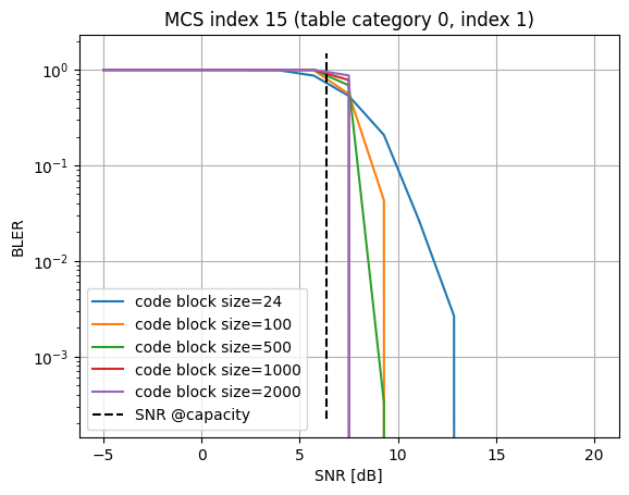
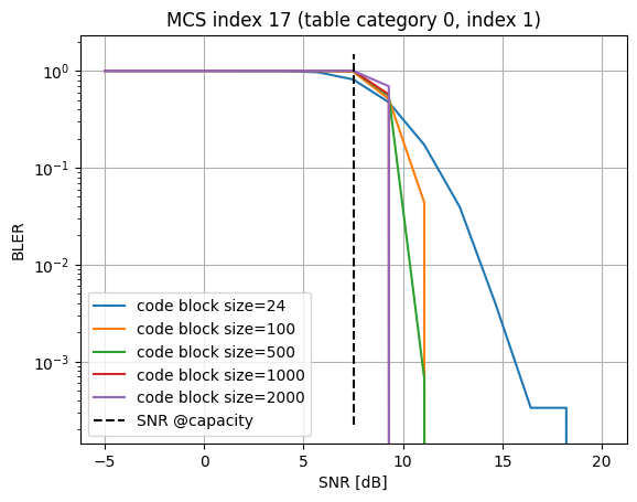
As can be seen from the figure above, the BLER depends not only depend on the MCS but also on the code block size (CBS). The longer the code, the lower the BLER.
Retrieve BLER values from interpolated tables
When a PHYAbstraction class is instantiated, the precomputed tables are interpolated over a fine two-dimensional grid of SINR and code block size (CBS) values. These interpolated tables are then used to obtain the BLER for different values of SINR and CBS.
The following code snippet shows this operation in detail. In general, you are not supposed to call this method directly, but rather use the call method of the PHYAbstraction class which does this for you, as shown later on.
This method also returns the transport block error rate (TBLER), which is the probability that at least one code block in a transport block is not decoded correctly.
[18]:
# Define the SNR and CB size at which BLER is retrieved
snr_eff_db = 9
cb_size = 80

# Compute the corresponding indices for the BLER interpolated table
snr_db_idx = phy_abs.get_idx_from_grid(snr_eff_db, 'snr')
cbs_idx = phy_abs.get_idx_from_grid(cb_size, 'cbs')

# Retrieve the interpolated BLER value
bler = phy_abs.bler_table_interp[mcs_category,
                                 mcs_table_index - 1,
                                 mcs_index,
                                 cbs_idx,
                                 snr_db_idx]

print(f'The BLER for MCS {mcs_index} at SNR {snr_eff_db} dB and CB size {cb_size} is {bler.numpy():.4f}')
The BLER for MCS 15 at SNR 9 dB and CB size 80 is 0.0511
Generate a new BLER table
For more details, see the documentation of the new_bler_table method and/or its source code.
[19]:
# Define MCS indices at which the new BLER table is simulated
sim_set = {'category': {
    1:  # 0 for PUSCH, 1 for PDSCH
    {'index': {
        2: {'MCS': [16]}
    }}}}

# SINR and Code Block size values at which new simulations are performed
sinr_dbs = np.linspace(5, 25, 25)
cb_sizes = [24, 200, 3000]

# Compute new BLER tables
new_table = phy_abs.new_bler_table(
    sinr_dbs,
    cb_sizes,
    sim_set,
    max_mc_iter=15,  # max n. Monte-Carlo iterations per SNR points
    batch_size=10,
    verbose=True)
BLER simulations started.
Total # (category, index, MCS, SINR) points to simulate: 3


Simulating category=1, index=2, CBS=24, MCS=16...

EbNo [dB] |        BER |       BLER |  bit errors |    num bits | block errors |  num blocks | runtime [s] |    status
---------------------------------------------------------------------------------------------------------------------------------------
   -1.246 | 2.6222e-01 | 1.0000e+00 |         944 |        3600 |          150 |         150 |         0.8 |reached max iterations
   -0.412 | 2.5417e-01 | 9.8667e-01 |         915 |        3600 |          148 |         150 |         0.4 |reached max iterations
    0.421 | 2.4778e-01 | 9.9333e-01 |         892 |        3600 |          149 |         150 |         0.5 |reached max iterations
    1.254 | 2.1000e-01 | 1.0000e+00 |         756 |        3600 |          150 |         150 |         0.5 |reached max iterations
    2.088 | 2.0056e-01 | 9.8667e-01 |         722 |        3600 |          148 |         150 |         0.4 |reached max iterations
    2.921 | 1.8944e-01 | 9.6000e-01 |         682 |        3600 |          144 |         150 |         0.5 |reached max iterations
    3.754 | 1.7667e-01 | 9.6000e-01 |         636 |        3600 |          144 |         150 |         0.4 |reached max iterations
    4.588 | 1.5972e-01 | 9.0000e-01 |         575 |        3600 |          135 |         150 |         0.4 |reached max iterations
    5.421 | 1.1722e-01 | 8.0667e-01 |         422 |        3600 |          121 |         150 |         0.4 |reached max iterations
    6.254 | 9.8333e-02 | 6.6667e-01 |         354 |        3600 |          100 |         150 |         0.5 |reached max iterations
    7.088 | 7.6389e-02 | 4.3333e-01 |         275 |        3600 |           65 |         150 |         0.4 |reached max iterations
    7.921 | 3.6667e-02 | 2.5333e-01 |         132 |        3600 |           38 |         150 |         0.4 |reached max iterations
    8.754 | 2.8056e-02 | 1.6000e-01 |         101 |        3600 |           24 |         150 |         0.5 |reached max iterations
    9.588 | 1.7222e-02 | 1.0667e-01 |          62 |        3600 |           16 |         150 |         0.5 |reached max iterations
   10.421 | 5.8333e-03 | 4.0000e-02 |          21 |        3600 |            6 |         150 |         0.4 |reached max iterations
   11.254 | 1.1111e-03 | 6.6667e-03 |           4 |        3600 |            1 |         150 |         0.5 |reached max iterations
   12.088 | 0.0000e+00 | 0.0000e+00 |           0 |        3600 |            0 |         150 |         0.5 |reached max iterations

Simulation stopped as no error occurred @ EbNo = 12.1 dB.


PROGRESS: 33.33%
Estimated remaining time: 0:00:16 [h:m:s]


Simulating category=1, index=2, CBS=200, MCS=16...

EbNo [dB] |        BER |       BLER |  bit errors |    num bits | block errors |  num blocks | runtime [s] |    status
---------------------------------------------------------------------------------------------------------------------------------------
   -1.246 | 2.5390e-01 | 1.0000e+00 |        7617 |       30000 |          150 |         150 |         0.8 |reached max iterations
   -0.412 | 2.4080e-01 | 1.0000e+00 |        7224 |       30000 |          150 |         150 |         0.5 |reached max iterations
    0.421 | 2.2620e-01 | 1.0000e+00 |        6786 |       30000 |          150 |         150 |         0.5 |reached max iterations
    1.254 | 2.1337e-01 | 1.0000e+00 |        6401 |       30000 |          150 |         150 |         0.5 |reached max iterations
    2.088 | 2.0313e-01 | 1.0000e+00 |        6094 |       30000 |          150 |         150 |         0.5 |reached max iterations
    2.921 | 1.8740e-01 | 1.0000e+00 |        5622 |       30000 |          150 |         150 |         0.4 |reached max iterations
    3.754 | 1.7140e-01 | 1.0000e+00 |        5142 |       30000 |          150 |         150 |         0.5 |reached max iterations
    4.588 | 1.5637e-01 | 1.0000e+00 |        4691 |       30000 |          150 |         150 |         0.5 |reached max iterations
    5.421 | 1.3770e-01 | 1.0000e+00 |        4131 |       30000 |          150 |         150 |         0.5 |reached max iterations
    6.254 | 1.1050e-01 | 9.9333e-01 |        3315 |       30000 |          149 |         150 |         0.4 |reached max iterations
    7.088 | 7.2367e-02 | 8.4667e-01 |        2171 |       30000 |          127 |         150 |         0.4 |reached max iterations
    7.921 | 4.3367e-02 | 5.8000e-01 |        1301 |       30000 |           87 |         150 |         0.4 |reached max iterations
    8.754 | 8.5667e-03 | 1.6667e-01 |         257 |       30000 |           25 |         150 |         0.5 |reached max iterations
    9.588 | 7.0000e-04 | 2.0000e-02 |          21 |       30000 |            3 |         150 |         0.5 |reached max iterations
   10.421 | 0.0000e+00 | 0.0000e+00 |           0 |       30000 |            0 |         150 |         0.5 |reached max iterations

Simulation stopped as no error occurred @ EbNo = 10.4 dB.


PROGRESS: 66.67%
Estimated remaining time: 0:00:07 [h:m:s]


Simulating category=1, index=2, CBS=3000, MCS=16...

EbNo [dB] |        BER |       BLER |  bit errors |    num bits | block errors |  num blocks | runtime [s] |    status
---------------------------------------------------------------------------------------------------------------------------------------
   -1.246 | 2.1102e-01 | 1.0000e+00 |       94957 |      450000 |          150 |         150 |         0.8 |reached max iterations
   -0.412 | 1.9497e-01 | 1.0000e+00 |       87738 |      450000 |          150 |         150 |         0.4 |reached max iterations
    0.421 | 1.8022e-01 | 1.0000e+00 |       81097 |      450000 |          150 |         150 |         0.4 |reached max iterations
    1.254 | 1.6595e-01 | 1.0000e+00 |       74677 |      450000 |          150 |         150 |         0.4 |reached max iterations
    2.088 | 1.5181e-01 | 1.0000e+00 |       68316 |      450000 |          150 |         150 |         0.4 |reached max iterations
    2.921 | 1.3863e-01 | 1.0000e+00 |       62383 |      450000 |          150 |         150 |         0.4 |reached max iterations
    3.754 | 1.2621e-01 | 1.0000e+00 |       56794 |      450000 |          150 |         150 |         0.4 |reached max iterations
    4.588 | 1.1146e-01 | 1.0000e+00 |       50157 |      450000 |          150 |         150 |         0.4 |reached max iterations
    5.421 | 9.6727e-02 | 1.0000e+00 |       43527 |      450000 |          150 |         150 |         0.4 |reached max iterations
    6.254 | 7.8140e-02 | 1.0000e+00 |       35163 |      450000 |          150 |         150 |         0.4 |reached max iterations
    7.088 | 4.9962e-02 | 1.0000e+00 |       22483 |      450000 |          150 |         150 |         0.4 |reached max iterations
    7.921 | 6.6133e-03 | 6.2667e-01 |        2976 |      450000 |           94 |         150 |         0.4 |reached max iterations
    8.754 | 0.0000e+00 | 0.0000e+00 |           0 |      450000 |            0 |         150 |         0.4 |reached max iterations

Simulation stopped as no error occurred @ EbNo = 8.8 dB.


PROGRESS: 100.00%
Estimated remaining time: 0:00:00 [h:m:s]


Simulations completed!
[20]:
# Plot the new BLER table
phy_abs.plot(plot_subset=sim_set,
             show=True);
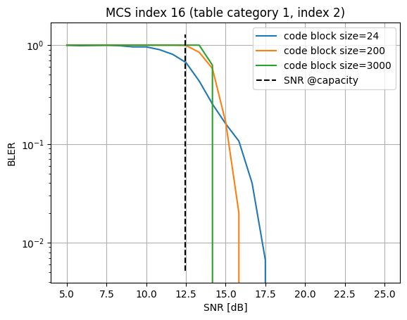
Please note that the new BLER table is overwritten to phy_abs.bler_table at the corresponding entries. We can also inspect the BLER table directly:
[21]:
new_table["category"][1]["index"][2]["MCS"][16]["CBS"][200]
[21]:
{'BLER': [1.0,
  1.0,
  1.0,
  1.0,
  1.0,
  1.0,
  1.0,
  1.0,
  1.0,
  0.9933333396911621,
  0.846666693687439,
  0.5799999833106995,
  0.1666666716337204,
  0.019999999552965164,
  0.0,
  0.0,
  0.0,
  0.0,
  0.0,
  0.0,
  0.0,
  0.0,
  0.0,
  0.0,
  0.0]}
Bypass physical layer computations
Once the PHYAbstraction object has been instantiated, we can use it to produce
Number of succesfully decoded bits;
Hybrid automatic repeat request (HARQ) value, reporting an ACK (HARQ=1) or a NACK (HARQ=0) depending on whether the transport block has been correctly received. If missing, -1 is reported;
Effective SINR value, that can be used as a measure of the channel condition quality for the user;
Block error rate (BLER), defining the probability that a code block is not decoded correctly;
Transport block error rate (TBLER), being the probability that at least one code block in a transport block is not decoded correctly.
We first set up the main parameters:
[22]:
# MCS table index
# Ranges within [1;4] for downlink and [1;2] for uplink, as in TS 38.214
mcs_table_index = 1

direction = 'uplink'  # 'downlink' or 'uplink'
mcs_category = int(direction == 'downlink')
num_ut = 80

# Time/frequency resource grid
num_ofdm_symbols = 14
num_subcarriers = 1024
num_streams_per_ut = 1

# BLER target value
bler_target = .1
[23]:
# Generate random SINR values across UT
# Target shape:
# […, num_ofdm_symbols, num_subcarriers, num_ut, num_streams_per_ut]
sinr_db = config.tf_rng.uniform([1,1,num_ut,1], minval=-5, maxval=30)

# Generate random SINR values across UT, subcarriers, and OFDM symbols
sinr_db = sinr_db + config.tf_rng.normal(
    [num_ofdm_symbols, num_subcarriers, num_ut, num_streams_per_ut], mean=0, stddev=2)
sinr = db_to_lin(sinr_db)
PHYAbstraction module also needs the MCS indices for each user.[24]:
illa = InnerLoopLinkAdaptation(phy_abs, bler_target)

mcs_index = illa(sinr=sinr,
                 mcs_table_index=mcs_table_index)
print("MCS indices: ",mcs_index.numpy())
MCS indices:  [14 18 10  5 27 23  7  5 13 27 25 27 24 23 12 27  5 27 19  2 16 17 27 27
 21 27 22 25  3 15 25 27 21  7 27  2 27  7 23 22  9 15 27 27 27 27 20 27
 27  7 21 16 16 17  5 27 25 12 27 23 27 16 27 27  3 12 27 27 27 17  4 27
 27 12 14 27  5 27 19 21]
We can now call the PHYAbstraction object, providing the generated per-stream SINR and per-user MCS index to obtain the number of decoded bits, HARQ feedback, effective SINR, BLER and TBLER.
Note that the transport block size is derived internally from the shape of the input per-stream SINR, revealing the number of allocated resources, and MCS index.
[25]:
# [batch_size, num_ut]
num_decoded_bits, harq_feedback, sinr_eff, bler, tbler = \
    phy_abs(mcs_index,
            sinr=sinr,
            mcs_table_index=mcs_table_index,
            mcs_category=mcs_category)

sinr_eff = sinr_eff.numpy()

# When HARQ feedback = 0, the Transport Block has not been decoded successfully
assert np.all(num_decoded_bits.numpy()[harq_feedback.numpy()==0]==0)

# Inspect the HARQ feedback
print("HARQ feedback: ", harq_feedback.numpy())
HARQ feedback:  [1 0 1 1 1 1 1 1 1 1 1 1 1 1 1 1 1 1 1 1 1 1 0 1 1 1 1 1 1 1 1 1 1 1 1 1 1
 1 1 1 1 1 1 1 1 1 1 1 1 1 1 1 1 1 1 1 1 1 1 1 1 1 1 1 1 1 1 1 1 1 1 1 1 1
 1 0 1 1 1 1]
Effective SINR
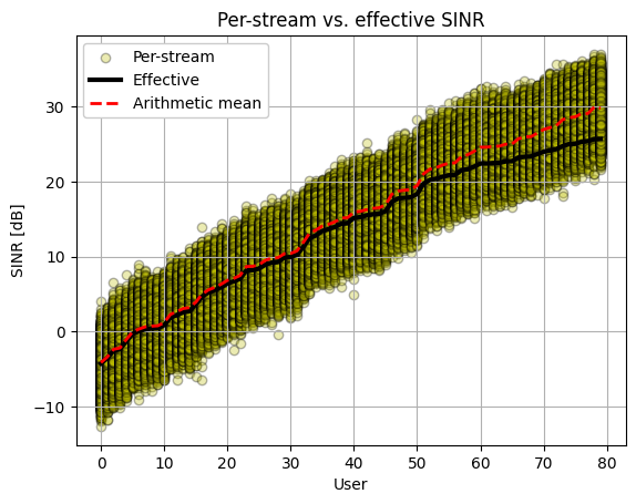
For a user experiencing a signal-to-interference-plus-noise ratio \(\mathrm{SINR}_i\) on time/frequency resource \(i=1,\dots,N\), its effective SINR is computed as:
where \(\beta>0\) is a parameter whose value depends on the used MCS.
It is interesting to visualize the relationship between the per-stream and the equivalent SINR for each user.
[26]:
# Sort users in increasing order of effective SINR
ind_sort = np.argsort(sinr_eff)

# [num_ut, num_ofdm_symbols, num_subcarriers, num_streams_per_ut]
sinr_t = np.transpose(sinr.numpy(), [2, 0, 1, 3])
# [num_ut, num_ofdm_symbols*num_subcarriers*num_streams_per_ut]
sinr_t = np.reshape(sinr_t, [num_ut, -1])
sinr_t = sinr_t[ind_sort, :]

# Visualize the effective vs. per-stream SINR values
fig, ax = plt.subplots()
for ut in range(num_ut):
    label = 'Per-stream' if ut==0 else None
    ax.scatter([ut]*sinr_t.shape[1], 10*np.log10(sinr_t[ut, :]), c='y', alpha=.3, edgecolors='k', label=label)
ax.plot(10*np.log10(sinr_eff[ind_sort]), '-k', linewidth=3, label='Effective')
ax.plot(10*np.log10(sinr_t.mean(axis=1)), '--r', linewidth=2, label='Arithmetic mean')
ax.set_xlabel('User')
ax.set_ylabel('SINR [dB]')
ax.set_title('Per-stream vs. effective SINR')
ax.grid()
ax.legend(framealpha=1)
plt.show()
Achieved vs. Shannon spectral efficiency
Finally, we compute the achieved spectral efficiency and compare it against the corresponding Shannon upper bound, for each user.
[27]:
# Determine if a resource element carries energy from at
# least one stream of a particular user
# [num_ofdm_sym, num_subcarriers, num_ut]
is_re_allocated = np.sum(sinr.numpy(), axis=-1) > 0

# Sum the number of allocated resource elements across
# all subcarriers and OFDM symbols
# [num_ut]
num_allocated_re = np.sum(is_re_allocated, axis=(-2, -3))

# Achieved spectral efficiency
# number of decoded bits of the transport block divided by the number of
# allocated resource elements
# [num_ut]
se_achieved = num_decoded_bits / num_allocated_re

# Shannon capacity
# [num_ut]
se_shannon = log2(tf.cast(1, sinr_eff.dtype) + sinr_eff)
[28]:
def get_cdf(values):
    """
    Computes the Cumulative Distribution Function (CDF) of the input vector
    """
    values = np.array(values).flatten()
    n = len(values)
    sorted_val = np.sort(values)
    cumulative_prob = np.arange(1, n+1) / n
    return sorted_val, cumulative_prob

fig, ax = plt.subplots(figsize=(5,4))
ind_sort = np.argsort(se_shannon.numpy())
ax.plot(se_achieved.numpy()[ind_sort], label='Achieved')
ax.plot(se_shannon.numpy()[ind_sort], label='Shannon bound')
ax.set_title('Spectral Efficiency')
ax.set_xlabel('User')
ax.set_ylabel('SE [bits/s/Hz]')
ax.legend()
ax.grid()
fig.tight_layout()
plt.show()
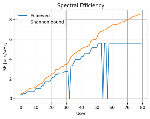
One can see that the achieved spectral efficiency is substantially lower than the Shannon capacity. At low SINR, this is mainly due to the fact that the targeted BLER limits the achievable spectral efficiency. At high SINR, the highest available MCS scheme is the main limiting factor. A zero spectral efficiency is observed when the transport block has not been decoded correctly, which occurs with probability TBLER.
You can play around with different BLER targets, MCS indices, tables, and resource grid sizes (i.e., number of OFDM symbols and subcarriers) to observe their impact on the achieved spectral efficiency.
Conclusions
The PHYAbstraction class bypasses the physical layer processing via the computation of an AWGN-equivalent effective SINR which is mapped to a BLER value according to precomputed tables.
SINR computation from OFDM channel matrices is covered in the hexagonal grid topology notebook;
Link adaptation for MCS selection is discussed in the link adaptation notebook.
References
[1] S. Lagen, K. Wanuga, H. Elkotby, S. Goyal, N. Patriciello, L. Giupponi. New radio physical layer abstraction for system-level simulations of 5G networks. IEEE International Conference on Communications (ICC), 2020