Radio Map Solvers

A radio map solver computes a radio map for a given Scene and for every Transmitter. Sionna provides a radio map solver (RadioMapSolver) which currently supports specular reflection (including specular chains), diffuse reflection, and refraction. It computes a path gain map, from which a received signal strength (RSS) map or a signal to interference plus noise ratio (SINR) map can be computed.

class sionna.rt.RadioMapSolver

Class that implements the radio map solver

This solver computes a radio map for every transmitter in the scene. For a given transmitter, a radio map is a rectangular surface with arbitrary orientation subdivded into rectangular cells of size $|C|=\mathtt{\text{cell\_size[0]}}\times \mathtt{\text{cell\_size[1]}}$. The parameter cell_size therefore controls the granularity of the map. The radio map associates with every cell $(i,j)$ the quantity

(54)$$g_{i,j}=\frac{1}{|C|}{\int }_{C_{i,j}}|h(s){|}^{2}ds$$

where $|h(s){|}^2$ is the squared amplitude of the path coefficients $a_i$ at position $s=(x,y)$ assuming an ideal isotropic receiver, the integral is over the cell $C_{i,j}$, and $ds$ is the infinitesimal small surface element $ds=dx\cdot dy$. The dimension indexed by $i$ ($j$) corresponds to the $y(x)$-axis of the radio map in its local coordinate system. The quantity $g_{i,j}$ can be seen as the average path_gain across a cell. This solver computes an approximation of $g_{i,j}$ through Monte Carlo integration.

The path gain can be transformed into the received signal strength (rss) by multiplying it with the transmit power:

$${\mathrm{RSS}}_{i,j}=P_{tx}{g}_{i,j}.$$

If a scene has multiple transmitters, the signal-to-interference-plus-noise ratio (sinr) for transmitter $k$ is then defined as

$${\mathrm{SINR}}_{i,j}^k=\frac{{\mathrm{RSS}}_{i,j}^k}{N_0+\sum _{k^{\prime }\ne k}{\mathrm{RSS}}_{i,j}^{k^{\prime }}}$$

where $N_0$ [W] is the thermal_noise_power, computed as:

$$N_0=B\times T\times k$$

where $B$ [Hz] is the transmission bandwidth, $T$ [K] is the temperature, and $k=1.380649\times {10}^{-23}$ [J/K] is the Boltzmann constant.

The output of this function is a real-valued matrix of size [num_cells_y, num_cells_x], for every transmitter, with elements equal to the sum of the contributions of paths, and where

$$\begin{array}{r}\mathtt{\text{num\_cells\_x}}=\lceil \frac{\mathtt{\text{size[0]}}}{\mathtt{\text{cell\_size[0]}}}\rceil \\ \mathtt{\text{num\_cells\_y}}=\lceil \frac{\mathtt{\text{size[1]}}}{\mathtt{\text{cell\_size[1]}}}\rceil .\end{array}$$

The surface defining the radio map is a rectangle centered at center, with orientation orientation, and with size size. An orientation of (0,0,0) corresponds to a radio map parallel to the XY plane, with surface normal pointing towards the $+z$ axis. By default, the radio map is parallel to the XY plane, covers all of the scene, and has an elevation of $z=1.5\text{m}$. If transmitter and has multiple antennas, transmit precoding is applied which is defined by precoding_vec.

For every ray $n$ intersecting the radio map cell $(i,j)$, the channel coefficients $a_n$ and the angles of departure (AoDs) $({\theta }_{\text{T},n},{\phi }_{\text{T},n})$ and arrival (AoAs) $({\theta }_{\text{R},n},{\phi }_{\text{R},n})$ are computed. See the Primer on Electromagnetics for more details.

A “synthetic” array is simulated by adding additional phase shifts that depend on the antenna position relative to the position of the transmitter as well as the AoDs. Let us denote by ${\mathbf{d}}_{\text{T},k}\in {\mathbb{R}}^3$ the relative position of the $k^{\text{th}}$ antenna (with respect to the position of the transmitter) for which the channel impulse response shall be computed. It can be accessed through the antenna array’s property positions. Using a plane-wave assumption, the resulting phase shift for this antenna can be computed as

$$p_{\text{T},n,k}=\frac{2\pi }{\lambda }\hat{\mathbf{r}}({\theta }_{\text{T},n},{\phi }_{\text{T},n}{)}^{\mathsf{T}}{\mathbf{d}}_{\text{T},k}.$$

The expression for the path coefficient of the $k\text{th}$ antenna is then

$$h_{n,k}=a_n{e}^{j{p}_{\text{T},n,k}}.$$

These coefficients form the complex-valued channel vector ${\mathbf{h}}_n$ of size $\mathtt{\text{num\_tx\_ant}}$.

Finally, the coefficient of the equivalent SISO channel is

$$h_n={\mathbf{h}}_n^{\mathsf{\text{H}}}\mathbf{p}$$

where $\mathbf{p}$ is the precoding vector precoding_vec.

Note

This solver supports Russian roulette, which can significantly improve the efficiency of ray tracing by terminating rays that contribute little to the final result.

The implementation of Russian roulette in this solver consists in terminating a ray with probability equal to the complement of its path gain (without the distance-based path loss). Formally, after the $d^{\text{th}}$ bounce, the ray path loss is set to:

$$\begin{array}{r}{a}_d\leftarrow \{\begin{array}{ll}\frac{a_d}{\sqrt{min\{p_c,|a_d{|}^2\}}},& \text{with probability }min\{p_c,|a_d{|}^2\}\\ 0,& \text{with probability }1-min\{p_c,|a_d{|}^2\}\end{array}\end{array}$$

where $a_d$ is the path coefficient corresponding to the ray (without the distance-based pathloss) and $p_c$ the maximum probability with which to continue a path (rr_prob). The first case consists in continuing the ray, whereas the second case consists in terminating the ray. When the ray is continued, the scaling by $\frac{1}{\sqrt{min\{p_c,|a_d{|}^2\}}}$ ensures an unbiased map by accounting for the rays that were terminated. When a ray is terminated, it is no longer traced, leading to a reduction of the required computations.

Russian roulette is by default disabled. It can be enabled by setting the rr_depth parameter to a positive value. rr_depth corresponds to the path depth, i.e., the number of bounces, from which on Russian roulette is enabled.

Note

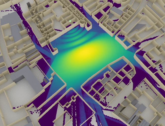
The parameter stop_threshold can be set to deactivate (i.e., stop tracing) paths whose gain has dropped below this threshold (in dB).

Example

import sionna
from sionna.rt import load_scene, PlanarArray, Transmitter, RadioMapSolver

scene = load_scene(sionna.rt.scene.munich)
scene.radio_materials["marble"].thickness = 0.5

# Configure antenna array for all transmitters
scene.tx_array = PlanarArray(num_rows=8,
                        num_cols=2,
                        vertical_spacing=0.7,
                        horizontal_spacing=0.5,
                        pattern="tr38901",
                        polarization="VH")

# Add a transmitters
tx = Transmitter(name="tx",
            position=[8.5,21,30],
            orientation=[0,0,0])
scene.add(tx)
tx.look_at(mi.Point3f(40,80,1.5))

solver = RadioMapSolver()
rm = solver(scene, cell_size=(1., 1.), samples_per_tx=100000000)
scene.preview(radio_map=rm, clip_at=15., rm_vmin=-100.)

__call__(scene, center=None, orientation=None, size=None, cell_size=[[10, 10]], precoding_vec=None, samples_per_tx=1000000, max_depth=3, los=True, specular_reflection=True, diffuse_reflection=False, refraction=True, seed=42, rr_depth=-1, rr_prob=0.95, stop_threshold=None)

Executes the solver

Parameters:

• scene (sionna.rt.scene.Scene) – Scene for which to compute the radio map

• center (typing.Optional[mitsuba.Point3f]) – Center of the radio map $(x,y,z)$ [m] as three-dimensional vector. If set to None, the radio map is centered on the center of the scene, except for the elevation $z$ that is set to 1.5m. Otherwise, orientation and size must be provided.

• orientation (typing.Optional[mitsuba.Point3f]) – Orientation of the radio map $(\alpha ,\beta ,\gamma )$ specified through three angles corresponding to a 3D rotation as defined in (3). An orientation of $(0,0,0)$ or None corresponds to a radio map that is parallel to the XY plane. If not set to None, then center and size must be provided.

• size (typing.Optional[mitsuba.Point2f]) – Size of the radio map [m]. If set to None, then the size of the radio map is set such that it covers the entire scene. Otherwise, center and orientation must be provided.

• cell_size (mitsuba.Point2f) – Size of a cell of the radio map [m]

• precoding_vec (typing.Optional[typing.Tuple[drjit.cuda.ad.TensorXf, drjit.cuda.ad.TensorXf]]) – Real and imaginary components of the complex-valued precoding vector. If set to None, then defaults to $\frac{1}{\sqrt{\text{num\_tx\_ant}}}[1,\dots ,1{]}^{\mathsf{T}}$.

• samples_per_tx (int) – Number of samples per source

• max_depth (int) – Maximum depth

• los (bool) – Enable line-of-sight paths

• specular_reflection (bool) – Enable specularl reflections

• diffuse_reflection (bool) – Enable diffuse reflectios

• refraction (bool) – Enable refraction

• seed (int) – Seed

• rr_depth (int) – Depth from which on to start Russian roulette

• rr_prob (float) – Maximum probability with which to keep a path when Russian roulette is enabled

• stop_threshold (typing.Optional[float]) – Gain threshold [dB] below which a path is deactivated

Return type:

sionna.rt.radio_map_solvers.radio_map.RadioMap

Returns:

Computed radio map

property loop_mode

Get/set the Dr.Jit mode used to evaluate the loop that implements the solver. Should be one of “evaluated” or “symbolic”. Symbolic mode (default) is the fastest one but does not support automatic differentiation. For more details, see the corresponding Dr.Jit documentation.

Type:

“evaluated” | “symbolic”