Custom Scattering Patterns

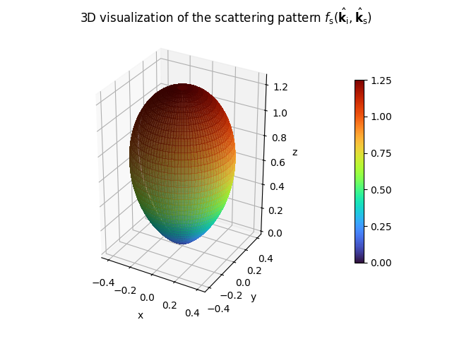
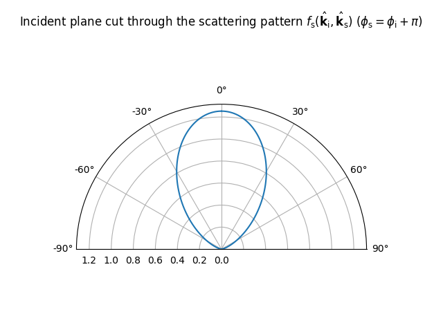
Similar to an antenna pattern, a scattering pattern describes the directivity of the diffusely reflected field. A detailed explanation can be found in the section “Scattering” of the EM Primer. In mathematical terms, it is described by a function

$$f({\hat{\mathbf{k}}}_{\text{i}},{\hat{\mathbf{k}}}_{\text{s}})\mapsto \mathbb{R}$$

where ${\hat{\mathbf{k}}}_{\text{i}}$ and ${\hat{\mathbf{k}}}_{\text{s}}$ are the directions of the incoming and outgoing rays, respectively. It is assumed that the latter are represented in the local coordinate system (or frame) of the corresponding surface element whose normal is pointing toward the positive $z$-axis.

If you want to add a new ScatteringPattern to Sionna RT, you must register a factory method for it together with a name, using the function register_scattering_pattern(). Once this is done, the new scattering pattern can be used everywhere by providing its name. An example is shown below:

import mitsuba as mi
import drjit as dr
from sionna.rt import RadioMaterial, ScatteringPattern, register_scattering_pattern

# Custom scattering pattern (only for illustration purposes)
class MyPattern(ScatteringPattern):
    """
    Custom scattering pattern implementing the function
    cos(theta_o)^n.
    """
    def __init__(self, n: int):
        self.n = n # Exponent
        self.normalization = dr.sqrt((n+1)/(2*dr.pi)) # Normalization constant

    def __call__(self, k_i_local, k_o_local):
        pattern = dr.sum(mi.Vector3f([0,0,1])*k_o_local, axis=0)**self.n
        return pattern * dr.rcp(self.normalization)

# Register new scattering pattern
register_scattering_pattern("my_pattern", MyPattern)

# Pattern can be referenced by its name
my_mat = RadioMaterial(name="my_material",
                    scattering_pattern="my_pattern", # Name of registered pattern
                    n=3) # Keyword argument passed to the class constructor

# Visualize the scattering pattern
my_mat.scattering_pattern.show()

Differentiable Parameters

Similar to what is shown in the guide on Gradient-based Optimization of antenna patterns, Dr.Jit can compute gradients of a loss function with respect to parameters of scattering patterns. This is shown in the next code snippet. Please note that this example is only meant for illustration purposes.

import mitsuba as mi
import drjit as dr
import sionna
from sionna.rt import RadioMaterial, ScatteringPattern, register_scattering_pattern,\
                      load_scene, Transmitter, Receiver, PlanarArray,\
                      PathSolver

# Custom scattering pattern with differentiable parameters
# Only meant for illustration purposes
class MyPattern(ScatteringPattern):
    """
    Custom scattering pattern implementing the function
    cos(theta_o)^n.
    """
    def __init__(self, n: int):
        self.n = n
        self.normalization = dr.sqrt((n+1)/(2*dr.pi))
        self.v = mi.Vector3f([0,0,1])
        dr.enable_grad(self.v) # Enable gradient computation for v

    def __call__(self, k_i_local, k_o_local):
        pattern = dr.sum(self.v*k_o_local, axis=0)**self.n
        return pattern * dr.rcp(self.normalization)

# Register new scattering pattern
register_scattering_pattern("my_pattern", MyPattern)

# Load scene, add transmitter and receiver
scene = load_scene(sionna.rt.scene.simple_reflector)
scene.add(Transmitter("tx", position=[-3,0,1.5]))
scene.add(Receiver("rx", position=[3,0,1.5]))
scene.tx_array = PlanarArray(num_cols=1, num_rows=1, pattern="iso", polarization="V")
scene.rx_array = scene.tx_array

# Create new radio material with custom scattering pattern
# and assign it to the reflector (only object in the scene)
my_mat = RadioMaterial(name="my_material",
                    conductivity=10,
                    relative_permittivity=5,
                    scattering_coefficient=0.8,
                    scattering_pattern="my_pattern",
                    n=3)

scene.get("merged-shapes").radio_material = my_mat

# Compute propagation paths
solver = PathSolver()

# Switch the computation of field loop to "evaluated" mode to
# enable gradient backpropagation through the loop
solver.loop_mode = "evaluated"

paths = solver(scene, diffuse_reflection=True) # Enable diffuse reflections

# Compute total received power
a_r, a_i = paths.a
power = dr.sum(a_r**2 + a_i**2)

# Compute gradients
dr.backward(power)

# Show gradient
print(my_mat.scattering_pattern.v.grad)

[[2.83798e-08, -6.06262e-11, 1.43508e-08]]