Sionna
  • Installation
    • Using pip
    • From source
    • Testing
    • Documentation
    • Developing
  • Ray Tracing (RT)
    • Tutorials
      • Introduction to Sionna RT
        • Imports
        • Loading and Visualizing Scenes
        • Inspecting SceneObjects and Editing of Scenes
        • Ray tracing of Propagation Paths
        • From Paths to Channel Impulse and Frequency Responses
        • Radio Maps
        • Summary
      • Tutorial on Mobility
        • Background Information
        • GPU Configuration and Imports
        • Controlling Position and Orientation of Scene Objects
        • Time Evolution of Channels Via Doppler Shift
          • Example: Delay-Doppler Spectrum
        • Comparison of Doppler- vs Position-based Time Evolution
        • Summary
      • Tutorial on Radio Maps
        • Imports
        • Understanding radio maps
          • Metrics
          • Multiple transmitters
          • User association
          • Sampling of random user positions
          • Directional antennas and precoding vectors
        • Radio map for a realistic scene
          • Channel impulse responses for random user locations
        • Conclusions
      • Tutorial on Scattering
        • Imports
        • Scattering Basics
        • Scattering Patterns
        • Validation Against the “Far”-Wall Approximation
        • Radio Maps With Scattering
        • Impact on Channel Impulse Response
        • Summary
        • References
      • Tutorial on Loading and Editing of Scenes
        • Imports
        • Loading Scenes and Merging Objects
        • Editing Scenes
        • Path Computation with the Edited Scene
        • Summary
    • Primer on Electromagnetics
      • Coordinate system, rotations, and vector fields
      • Planar Time-Harmonic Waves
      • Far Field of a Transmitting Antenna
      • Modelling of a Receiving Antenna
      • General Propagation Path
      • Frequency & Impulse Response
      • Reflection and Refraction
        • Single-layer Slab
      • Diffraction
      • Scattering
      • Reconfigurable Intelligent Surfaces (RIS)
    • API Documentation
      • Antenna Arrays
        • AntennaArray
          • AntennaArray.antenna_pattern
          • AntennaArray.array_size
          • AntennaArray.normalized_positions
          • AntennaArray.num_ant
          • AntennaArray.positions()
          • AntennaArray.rotate()
        • PlanarArray
          • PlanarArray.antenna_pattern
          • PlanarArray.array_size
          • PlanarArray.normalized_positions
          • PlanarArray.num_ant
          • PlanarArray.positions()
          • PlanarArray.rotate()
          • PlanarArray.show()
      • Antenna Patterns
        • AntennaPattern
          • AntennaPattern.compute_gain()
          • AntennaPattern.patterns
          • AntennaPattern.show()
        • PolarizedAntennaPattern
          • PolarizedAntennaPattern.compute_gain()
          • PolarizedAntennaPattern.patterns
          • PolarizedAntennaPattern.show()
        • Vertically Polarized Antenna Pattern Functions
          • v_iso_pattern()
          • v_dipole_pattern()
          • v_hw_dipole_pattern()
          • v_tr38901_pattern()
        • Polarization Models
          • polarization_model_tr38901_1()
          • polarization_model_tr38901_2()
        • Utility Functions
          • antenna_pattern_to_world_implicit()
          • complex2real_antenna_pattern()
          • register_antenna_pattern()
          • register_polarization()
          • register_polarization_model()
      • Cameras
        • Camera
          • Camera.look_at()
          • Camera.orientation
          • Camera.position
      • Paths
        • Paths
          • Paths.a
          • Paths.cfr()
          • Paths.cir()
          • Paths.doppler
          • Paths.interactions
          • Paths.num_rx
          • Paths.num_tx
          • Paths.objects
          • Paths.phi_r
          • Paths.phi_t
          • Paths.primitives
          • Paths.rx_array
          • Paths.sources
          • Paths.synthetic_array
          • Paths.taps()
          • Paths.targets
          • Paths.tau
          • Paths.theta_r
          • Paths.theta_t
          • Paths.tx_array
          • Paths.valid
          • Paths.vertices
        • Constants
          • InteractionType
          • INVALID_SHAPE
          • INVALID_PRIMITIVE
      • Path Solvers
        • PathSolver
          • PathSolver.__call__()
          • PathSolver.loop_mode
      • Radio Devices
        • RadioDevice
          • RadioDevice.color
          • RadioDevice.display_radius
          • RadioDevice.look_at()
          • RadioDevice.name
          • RadioDevice.orientation
          • RadioDevice.position
          • RadioDevice.velocity
        • Receiver
        • Transmitter
          • Transmitter.power
          • Transmitter.power_dbm
      • Radio Map
        • RadioMap
          • RadioMap.cdf()
          • RadioMap.cell_centers
          • RadioMap.cell_size
          • RadioMap.center
          • RadioMap.num_cells
          • RadioMap.num_rx
          • RadioMap.num_tx
          • RadioMap.orientation
          • RadioMap.path_gain
          • RadioMap.rss
          • RadioMap.rx_cell_indices
          • RadioMap.sample_positions()
          • RadioMap.show()
          • RadioMap.show_association()
          • RadioMap.sinr
          • RadioMap.size
          • RadioMap.tx_association()
          • RadioMap.tx_cell_indices
      • Radio Map Solvers
        • RadioMapSolver
          • RadioMapSolver.__call__()
          • RadioMapSolver.loop_mode
      • Radio Materials
        • RadioMaterialBase
          • RadioMaterialBase.color
          • RadioMaterialBase.eval()
          • RadioMaterialBase.name
          • RadioMaterialBase.pdf()
          • RadioMaterialBase.sample()
          • RadioMaterialBase.scene
          • RadioMaterialBase.to_string()
          • RadioMaterialBase.traverse()
        • RadioMaterial
          • RadioMaterial.conductivity
          • RadioMaterial.frequency_update()
          • RadioMaterial.frequency_update_callback
          • RadioMaterial.relative_permittivity
          • RadioMaterial.scattering_coefficient
          • RadioMaterial.scattering_pattern
          • RadioMaterial.thickness
          • RadioMaterial.xpd_coefficient
        • ITURadioMaterial
          • ITURadioMaterial.itu_type
          • ITURadioMaterial.to_string()
        • HolderMaterial
          • HolderMaterial.radio_material
          • HolderMaterial.velocity
        • Scattering Patterns
          • ScatteringPattern
          • LambertianPattern
          • DirectivePattern
          • BackscatteringPattern
          • register_scattering_pattern()
      • Scenes
        • load_scene()
        • Scene
          • Scene.add()
          • Scene.all_set()
          • Scene.angular_frequency
          • Scene.bandwidth
          • Scene.edit()
          • Scene.frequency
          • Scene.get()
          • Scene.mi_scene
          • Scene.mi_scene_params
          • Scene.objects
          • Scene.paths_solver
          • Scene.preview()
          • Scene.radio_materials
          • Scene.receivers
          • Scene.remove()
          • Scene.render()
          • Scene.render_to_file()
          • Scene.rx_array
          • Scene.scene_geometry_updated()
          • Scene.sources()
          • Scene.targets()
          • Scene.temperature
          • Scene.thermal_noise_power
          • Scene.transmitters
          • Scene.tx_array
          • Scene.wavelength
        • Examples
          • box
          • box_one_screen
          • box_two_screens
          • double_reflector
          • etoile
          • floor_wall
          • florence
          • munich
          • simple_reflector
          • simple_street_canyon
          • simple_street_canyon_with_cars
          • simple_wedge
          • triple_reflector
      • Scene Objects
        • SceneObject
          • SceneObject.look_at()
          • SceneObject.mi_shape
          • SceneObject.name
          • SceneObject.object_id
          • SceneObject.orientation
          • SceneObject.position
          • SceneObject.radio_material
          • SceneObject.scaling
          • SceneObject.scene
          • SceneObject.velocity
      • Utility Functions
        • Complex-valued tensors
          • cpx_abs()
          • cpx_abs_square()
          • cpx_add()
          • cpx_convert()
          • cpx_div()
          • cpx_exp()
          • cpx_mul()
          • cpx_sqrt()
          • cpx_sub()
        • Electromagnetics
          • complex_relative_permittivity()
          • fresnel_reflection_coefficients_simplified()
          • itu_coefficients_single_layer_slab()
        • Geometry
          • phi_hat()
          • theta_hat()
          • r_hat()
          • theta_phi_from_unit_vec()
          • rotation_matrix()
        • Jones calculus
          • implicit_basis_vector()
          • jones_matrix_rotator()
          • jones_matrix_rotator_flip_forward()
          • to_world_jones_rotator()
          • jones_matrix_to_world_implicit()
          • jones_vec_dot()
        • Miscellaneous
          • complex_sqrt()
          • dbm_to_watt()
          • isclose()
          • log10()
          • sigmoid()
          • sinc()
          • subcarrier_frequencies()
          • watt_to_dbm()
        • Ray tracing
          • fibonacci_lattice()
          • spawn_ray_from_sources()
          • offset_p()
          • spawn_ray_towards()
          • spawn_ray_to()
    • Developer Guides
      • Compatibility with other Frameworks
        • Type conversions
        • Gradients
        • Training-Loop in PyTorch
      • Understanding the Paths Object
      • Custom Antenna Patterns
        • Gradient-based Optimization
      • Understanding Radio Materials
        • Modifying Parameters of Radio Materials
        • Calibrating Material Parameters Through Gradient Descent
        • Custom Radio Materials
          • Representation of Jones vector and Matrices
          • Implicit Basis
          • The Local Interaction Basis
          • Mandatory Subclass Methods
          • Implementation of a Simple Radio Material Model
          • A More Complex Material Model
      • Custom Scattering Patterns
        • Differentiable Parameters
    • Technical Report
  • Physical Layer (PHY)
    • Tutorials
      • Beginners
        • “Hello, world!”
        • Part 1: Getting Started with Sionna
          • Imports & Basics
          • A note on random number generation
          • Sionna Data-flow and Design Paradigms
          • Hello, Sionna!
          • Communication Systems as Sionna Blocks
          • Forward Error Correction (FEC)
          • Eager vs Graph Mode
          • Exercise
        • Part 2: Differentiable Communication Systems
          • Imports
          • Gradient Computation Through End-to-end Systems
          • Creating Custom Layers
          • Setting up Training Loops
        • Part 3: Advanced Link-level Simulations
          • Imports
          • OFDM Resource Grid and Stream Management
          • Antenna Arrays
          • Channel Model
          • Uplink Transmission in the Frequency Domain
        • Part 4: Toward Learned Receivers
          • Imports
          • Simulation Parameters
          • Implemention of an Advanced Neural Receiver
          • Training the Neural Receiver
          • Benchmarking the Neural Receiver
          • Conclusion
          • References
        • Basic MIMO Simulations
          • Table of Contents
          • Simple uncoded transmission
          • Extension to channel coding
        • Pulse-shaping Basics
          • Table of Contents
          • GPU Configuration and Imports
          • Pulse-shaping of a sequence of QAM symbols
          • Recovering the QAM symbols through matched filtering and downsampling
          • Investigating the ACLR
          • Windowing
        • Optical Channel with Lumped Amplification
          • Table of Contents
          • Setup
          • Impulse Generation
          • Attenuation
          • Amplified Spontaneous Emission Noise
          • Chromatic Dispersion
          • Kerr Nonlinearity
          • Split-Step Fourier Method
          • References
      • Experts
        • 5G Channel Coding and Rate-Matching: Polar vs. LDPC Codes
          • Table of Contents
          • GPU Configuration and Imports
          • BER Performance of 5G Coding Schemes
          • A Deeper Look into the Polar Code Module
          • Rate-Matching and Rate-Recovery
          • Throughput and Decoding Complexity
          • References
        • 5G NR PUSCH Tutorial
          • Table of Contents
          • GPU Configuration and Imports
          • A Hello World Example
          • Carrier Configuration
          • Understanding the DMRS Configuration
          • Transport Blocks and MCS
          • Looking into the PUSCHTransmitter
          • Components of the PUSCHReceiver
          • End-to-end PUSCH Simulations
        • Bit-Interleaved Coded Modulation (BICM)
          • Table of Contents
          • System Block Diagram
          • GPU Configuration and Imports
          • A Simple BICM System
          • All-zero Codeword Simulations
          • EXIT Charts
          • Mismatched Demapping and the Advantages of Min-sum Decoding
          • References
        • MIMO OFDM Transmissions over the CDL Channel Model
          • Table of Contents
          • System Setup
          • Simulations
        • Neural Receiver for OFDM SIMO Systems
          • GPU Configuration and Imports
          • Simulation Parameters
          • Neural Receiver
          • End-to-end System
          • End-to-end System as a Sionna Block
          • Evaluation of the Baselines
          • Training the Neural Receiver
          • Evaluation of the Neural Receiver
          • Pre-computed Results
          • References
        • Realistic Multiuser MIMO OFDM Simulations
          • Table of Contents
          • GPU Configuration and Imports
          • System Setup
          • Uplink Transmissions in the Frequency Domain
        • OFDM MIMO Channel Estimation and Detection
          • Table of Contents
          • GPU Configuration and Imports
          • Simulation parameters
          • Estimation of the channel time, frequency, and spatial covariance matrices
          • Loading the channel covariance matrices
          • Comparison of OFDM estimators
          • Comparison of MIMO detectors
        • Introduction to Iterative Detection and Decoding
          • Iterative Detection and Decoding
          • Table of contents
          • GPU Configuration and Imports
          • Simulation Parameters
          • Setting-up an End-to-end Block
          • Non-IDD versus IDD Benchmarks
          • Discussion-Optimizing IDD with Machine Learning
          • Comments
          • List of References
        • End-to-end Learning with Autoencoders
          • GPU Configuration and Imports
          • Simulation Parameters
          • Neural Demapper
          • Trainable End-to-end System: Conventional Training
          • Trainable End-to-end System: RL-based Training
          • Evaluation
          • Visualizing the Learned Constellations
          • References
        • Weighted Belief Propagation Decoding
          • Table of Contents
          • GPU Configuration and Imports
          • Weighted BP for BCH Codes
          • Further Experiments
          • References
        • Channel Models from Datasets
          • GPU Configuration and Imports
          • Simulation Parameters
          • Creating a Simple Dataset
          • Generators
          • Use the Channel Model for OFDM Transmissions
        • Using the DeepMIMO Dataset with Sionna
          • Table of Contents
          • GPU Configuration and Imports
          • Configuration of DeepMIMO
          • Using DeepMIMO with Sionna
          • Link-level Simulations using Sionna and DeepMIMO
          • DeepMIMO License and Citation
        • Link-level simulations with Sionna RT
          • Background Information
          • Imports
          • Setting up the Ray Tracer
          • Creating a CIR Dataset
          • PUSCH Link-Level Simulations
    • API Documentation
      • Configuration
        • Config
          • Config.np_cdtype
          • Config.np_rdtype
          • Config.np_rng
          • Config.precision
          • Config.py_rng
          • Config.seed
          • Config.tf_cdtype
          • Config.tf_rdtype
          • Config.tf_rng
      • Forward Error Correction (FEC)
        • Linear Codes
          • LinearEncoder
          • OSDecoder
        • Low-Density Parity-Check (LDPC)
          • LDPC5GEncoder
          • LDPCBPDecoder
          • LDPC5GDecoder
          • Node Update Functions
          • Decoder Callbacks
        • Polar Codes
          • Polar5GEncoder
          • PolarEncoder
          • Polar5GDecoder
          • PolarSCDecoder
          • PolarSCLDecoder
          • PolarBPDecoder
          • Utility Functions
        • Convolutional Codes
          • ConvEncoder
          • ViterbiDecoder
          • BCJRDecoder
          • Utility Functions
        • Turbo Codes
          • TurboEncoder
          • TurboDecoder
          • Utility Functions
        • Cyclic Redundancy Check (CRC)
          • CRCEncoder
          • CRCDecoder
        • Interleaving
          • RowColumnInterleaver
          • RandomInterleaver
          • Turbo3GPPInterleaver
          • Deinterleaver
        • Scrambling
          • Scrambler
          • TB5GScrambler
          • Descrambler
        • Utility Functions
          • (Binary) Linear Codes
          • EXIT Analysis
          • Miscellaneous
      • Mapping
        • Constellation
          • Constellation.center
          • Constellation.constellation_type
          • Constellation.normalize
          • Constellation.num_bits_per_symbol
          • Constellation.num_points
          • Constellation.points
          • Constellation.show()
        • Mapper
          • Mapper.constellation
        • Demapper
          • Demapper.constellation
        • SymbolDemapper
        • Utility Functions
          • BinarySource
          • LLRs2SymbolLogits
          • PAMSource
          • PAM2QAM
          • QAMSource
          • QAM2PAM
          • SymbolInds2Bits
          • SymbolLogits2LLRs
          • SymbolLogits2Moments
          • SymbolSource
      • Wireless Channel Models
        • AWGN
        • Flat-fading channel
          • FlatFadingChannel
          • GenerateFlatFadingChannel
          • ApplyFlatFadingChannel
          • SpatialCorrelation
          • KroneckerModel
          • PerColumnModel
        • Channel model interface
          • ChannelModel
        • Time domain channel
          • TimeChannel
          • GenerateTimeChannel
          • ApplyTimeChannel
          • cir_to_time_channel()
          • time_to_ofdm_channel()
        • Channel with OFDM waveform
          • OFDMChannel
          • GenerateOFDMChannel
          • ApplyOFDMChannel
          • cir_to_ofdm_channel()
        • Rayleigh block fading
          • RayleighBlockFading
        • 3GPP 38.901 channel models
          • PanelArray
          • Antenna
          • AntennaArray
          • TDL
          • CDL
          • UMi
          • UMa
          • RMa
        • External datasets
          • CIRDataset
        • Utility functions
          • subcarrier_frequencies()
          • time_lag_discrete_time_channel()
          • deg_2_rad()
          • rad_2_deg()
          • wrap_angle_0_360()
          • drop_uts_in_sector()
          • relocate_uts()
          • set_3gpp_scenario_parameters()
          • gen_single_sector_topology()
          • gen_single_sector_topology_interferers()
          • exp_corr_mat()
          • one_ring_corr_mat()
      • Optical Channel Models
        • SSFM
        • EDFA
        • Utility functions
          • time_frequency_vector()
      • Discrete Channel Models
        • BinaryErasureChannel
        • BinaryMemorylessChannel
          • BinaryMemorylessChannel.llr_max
          • BinaryMemorylessChannel.temperature
        • BinarySymmetricChannel
        • BinaryZChannel
      • Orthogonal Frequency-Division Multiplexing (OFDM)
        • Resource Grid
          • ResourceGrid
          • ResourceGridMapper
          • ResourceGridDemapper
          • RemoveNulledSubcarriers
        • Modulation & Demodulation
          • OFDMModulator
          • OFDMDemodulator
        • Pilot Pattern
          • PilotPattern
          • EmptyPilotPattern
          • KroneckerPilotPattern
        • Channel Estimation
          • BaseChannelEstimator
          • BaseChannelInterpolator
          • LSChannelEstimator
          • LinearInterpolator
          • LMMSEInterpolator
          • NearestNeighborInterpolator
          • tdl_time_cov_mat()
          • tdl_freq_cov_mat()
        • Precoding
          • RZFPrecoder
          • PrecodedChannel
          • CBFPrecodedChannel
          • EyePrecodedChannel
          • RZFPrecodedChannel
        • Equalization
          • OFDMEqualizer
          • LMMSEEqualizer
          • MFEqualizer
          • ZFEqualizer
          • PostEqualizationSINR
          • LMMSEPostEqualizationSINR
        • Detection
          • OFDMDetector
          • OFDMDetectorWithPrior
          • EPDetector
          • KBestDetector
          • LinearDetector
          • MaximumLikelihoodDetector
          • MaximumLikelihoodDetectorWithPrior
          • MMSEPICDetector
      • Multiple-Input Multiple-Output (MIMO)
        • Stream Management
          • StreamManagement
        • Precoding
          • cbf_precoding_matrix()
          • rzf_precoding_matrix()
          • rzf_precoder()
          • grid_of_beams_dft_ula()
          • grid_of_beams_dft()
          • flatten_precoding_mat()
          • normalize_precoding_power()
        • Equalization
          • lmmse_matrix()
          • lmmse_equalizer()
          • mf_equalizer()
          • zf_equalizer()
        • Detection
          • EPDetector
          • KBestDetector
          • LinearDetector
          • MaximumLikelihoodDetector
          • MMSEPICDetector
        • Utility Functions
          • List2LLR
          • List2LLRSimple
          • complex2real_vector()
          • real2complex_vector()
          • complex2real_matrix()
          • real2complex_matrix()
          • complex2real_covariance()
          • real2complex_covariance()
          • complex2real_channel()
          • real2complex_channel()
          • whiten_channel()
      • 5G NR
        • Carrier
          • CarrierConfig
        • Layer Mapping
          • LayerMapper
          • LayerDemapper
        • PUSCH
          • PUSCHConfig
          • PUSCHDMRSConfig
          • PUSCHLSChannelEstimator
          • PUSCHPilotPattern
          • PUSCHPrecoder
          • PUSCHReceiver
          • PUSCHTransmitter
        • Transport Block
          • TBConfig
          • TBEncoder
          • TBDecoder
        • Utils
          • calculate_tb_size()
          • generate_prng_seq()
          • decode_mcs_index()
          • calculate_num_coded_bits()
          • TransportBlockNR
          • CodedAWGNChannelNR
          • MCSDecoderNR
      • Signal
        • Filters
          • SincFilter
          • RaisedCosineFilter
          • RootRaisedCosineFilter
          • CustomFilter
          • Filter
        • Window functions
          • HannWindow
          • HammingWindow
          • BlackmanWindow
          • CustomWindow
          • Window
        • Utility Functions
          • convolve()
          • fft()
          • ifft()
          • Upsampling
          • Downsampling
          • empirical_psd()
          • empirical_aclr()
      • Utility Functions
        • Linear Algebra
          • inv_cholesky()
          • matrix_pinv()
        • Metrics
          • compute_ber()
          • compute_bler()
          • compute_ser()
          • count_block_errors()
          • count_errors()
        • Miscellaneous
          • dbm_to_watt()
          • db_to_lin
          • DeepUpdateDict
          • dict_keys_to_int()
          • ebnodb2no()
          • complex_normal()
          • hard_decisions()
          • Interpolate
          • lin_to_db
          • log2()
          • log10()
          • MCSDecoder
          • scalar_to_shaped_tensor()
          • sim_ber()
          • SingleLinkChannel
          • SplineGriddataInterpolation
          • to_list()
          • TransportBlock
          • watt_to_dbm()
        • Numerics
          • bisection_method()
        • Plotting
          • plot_ber()
          • PlotBER
        • Tensors
          • expand_to_rank()
          • flatten_dims()
          • flatten_last_dims()
          • insert_dims()
          • split_dim()
          • diag_part_axis()
          • flatten_multi_index()
          • gather_from_batched_indices()
          • tensor_values_are_in_set()
          • enumerate_indices()
      • For Developers
        • Object
          • Object.cdtype
          • Object.precision
          • Object.rdtype
        • Block
          • Block.build()
          • Block.built
          • Block.call()
    • Developer Guides
      • Matrix inversion
        • Solving linear systems
        • Correlated random vectors
      • Random number generation
      • Sionna Block and Object
        • Understanding Sionna Blocks
  • System Level (SYS)
    • Tutorials
      • Beginners
        • Physical Layer Abstraction
          • Imports
          • Instantiate a PHYAbstraction object
          • Retrieve BLER values from interpolated tables
          • Generate a new BLER table
          • Bypass physical layer computations
          • Effective SINR
          • Conclusions
          • References
        • Link Adaptation
          • Imports
          • Simulation parameters
          • The principles of link adaptation
          • Inner-Loop Link Adaptation (ILLA)
          • Outer-Loop Link Adaption (OLLA)
          • Conclusions
          • References
        • Proportional Fairness Scheduler
          • Imports
          • The main principle
          • Basic scenario
          • Schedule users
          • Evaluate performance
          • Conclusions
          • References
        • Hexagonal Grid Topology
          • Imports
          • Generate a multicell topology
          • Drop users
          • Set up a 3GPP multicell scenario
          • Per-stream SINR computation
          • Conclusions
        • Power Control
          • Imports
          • Multicell scenario
          • Uplink power control
          • Downlink power control
          • Conclusions
          • References
      • Experts
        • Sionna SYS meets Sionna RT
          • Imports
          • Simulation parameters
          • Scene creation
          • Channel generation via Sionna RT
          • System-level simulation
          • Conclusions
        • System-Level Simulations
          • Imports
          • Utils
          • Simulation
          • Performance metric analysis
          • Conclusions
    • API Documentation
      • PHY Abstraction
        • EffectiveSINR
          • EffectiveSINR.calibrate()
        • EESM
          • EESM.beta_table
          • EESM.beta_table_filenames
          • EESM.beta_tensor
          • EESM.validate_beta_table()
        • PHYAbstraction
          • PHYAbstraction.bler_interp_delta
          • PHYAbstraction.bler_table
          • PHYAbstraction.bler_table_filenames
          • PHYAbstraction.bler_table_interp
          • PHYAbstraction.cbs_interp_min_max_delta
          • PHYAbstraction.get_bler()
          • PHYAbstraction.get_idx_from_grid()
          • PHYAbstraction.load_table()
          • PHYAbstraction.new_bler_table()
          • PHYAbstraction.plot()
          • PHYAbstraction.snr_db_interp_min_max_delta
          • PHYAbstraction.snr_table_interp
          • PHYAbstraction.validate_bler_table()
      • Link Adaptation
        • InnerLoopLinkAdaptation
          • InnerLoopLinkAdaptation.bler_target
        • OuterLoopLinkAdaptation
          • OuterLoopLinkAdaptation.bler_target
          • OuterLoopLinkAdaptation.delta_down
          • OuterLoopLinkAdaptation.delta_up
          • OuterLoopLinkAdaptation.offset
          • OuterLoopLinkAdaptation.offset_max
          • OuterLoopLinkAdaptation.offset_min
          • OuterLoopLinkAdaptation.reset()
          • OuterLoopLinkAdaptation.sinr_eff_db_last
        • Note
      • Power Control
        • Uplink
          • open_loop_uplink_power_control()
        • Downlink
          • downlink_fair_power_control()
      • Scheduling
        • PFSchedulerSUMIMO
          • PFSchedulerSUMIMO.beta
          • PFSchedulerSUMIMO.pf_metric
          • PFSchedulerSUMIMO.rate_achieved_past
      • Multicell Topology
        • Hexagon
          • Hexagon.coord_axial
          • Hexagon.coord_dict()
          • Hexagon.coord_euclid
          • Hexagon.coord_offset
          • Hexagon.corners()
          • Hexagon.neighbor()
          • Hexagon.radius
        • HexGrid
          • HexGrid.cell_height
          • HexGrid.cell_loc
          • HexGrid.cell_radius
          • HexGrid.center_loc
          • HexGrid.grid
          • HexGrid.isd
          • HexGrid.mirror_cell_loc
          • HexGrid.num_cells
          • HexGrid.num_rings
          • HexGrid.show()
        • gen_hexgrid_topology()
        • get_num_hex_in_grid()
        • convert_hex_coord()
      • Utils
        • get_pathloss()
        • is_scheduled_in_slot()
        • spread_across_subcarriers()
  • Research Kit (RK)
    • Quickstart
      • Hardware Requirements
      • Step 1: Jetson Setup
      • Step 2: USRP Setup
      • Step 3: UE Setup
      • Step 4: Deploy 5G Stack
      • Have Your First Call
    • Setup
      • Platform Preparation
        • Bill of Materials
          • Computing Platform
          • RF Components
          • User Equipment
          • Optional Components
        • Jetson Setup
          • OS Installation
          • Post-Installation Setup
          • Version Information
        • Custom Linux Kernel
          • Prerequisites
          • Source Code
          • Kernel Configuration
          • Building the Kernel
          • Installing Kernel Image and Modules
          • Configure Boot Sequence
        • Performance Tweaks
          • Power Management
          • Default System Mode
          • Real-Time Scheduling
          • Verifying Settings
        • USRP Driver Installation
          • Key Resources
          • Prerequisites
          • Building UHD
          • Post-build Configuration
          • Testing Installation
        • SIM Card Programming
          • Prerequisites
          • UICC Software Setup
          • Programming SIM Card
          • Additional Resources
        • Quectel Modem Setup
          • Basic Configuration
          • AT Command Reference
          • Additional Resources
      • Software Configuration
        • OpenAirInterface Setup
          • Required Components
          • TLDR
          • Getting the Source Code
          • Patching
          • Create configuration files
          • Building OAI RAN Images
          • Building OAI 5G Core Images
          • Building Components Manually
        • 5G System Configuration
          • Environment Variables
          • Additional Resources
        • Using RF Simulator Mode
          • Basic Configuration
          • Dynamic Re-configuration
        • Installing Sionna
      • Your First Call
        • Connect & Test Performance
      • Documentation of Scripts
        • Setup Scripts
          • quickstart-oai.sh
          • quickstart-cn5g.sh
          • configure-system.sh
          • install-usrp.sh
        • Linux Kernel Customization
          • build-custom-kernel.sh
          • install-custom-kernel.sh
        • Configuration Files
          • start-system.sh
          • stop-system.sh
          • generate-configs.sh
        • Building Docker Images
          • build-cn5g-images.sh
          • build-oai-images.sh
        • Development / Patch tracking
          • get-config-changes.sh
          • get-oai-changed-files.sh
          • get-oai-cn5g-changed-files.sh
          • get-oai-commit-versions.sh
          • get-oai-cn5g-commit-versions.sh
    • Tutorials
      • Running the Tutorials
        • Command Cheat-sheet
        • GPU-Accelerated LDPC
        • Demapper Plugin
        • Data Capture Plugin
        • TensorRT Neural Demapper
      • GPU-Accelerated LDPC Decoding
        • Part 1: Background & Python Reference Implementation
          • Background: Channel Coding in 5G
          • Overview Decoder Implementation
          • Memory Layout
          • CN Update Function
          • VN Update Function
          • Hard-decision
          • Main Decoding Function
          • Run and Test the Decoder
        • Part 2: CUDA Implementation
          • Overview
          • CUDA Integration in OAI
          • Running the Decoder
          • Implementation Aspects
          • Outlook - Weighted Belief Propagation
        • References
      • Plugins & Data Acquisition
        • Part 1: Create a Plugin
          • Architecture Overview
          • Select Functions
          • Define Module Interface
          • Loading the Module
          • Use Module Functions
          • Module Implementation
          • Compiling
          • Incremental Builds
          • Container Changes
        • Part 2: Capture Data
          • Adding New Plugin Variant
          • Using New Plugin Variant
          • Access Captured Files
          • Capture Format
          • Add Timestamps
          • Account for Multi-Threading
          • Final Source Code
        • References
      • Integration of a Neural Demapper
        • Part 1: Neural Demapper Training and TensorRT Export
          • Python Imports
          • Background: APP-Demapping
          • Understanding the OAI Data Structure
          • Neural Demapper
          • Blind Demapping & Training with Synthetic Data
          • Improved Demapping & Training with Captured Data
          • Export TensorRT Engine
        • Part 2: GPU-Accelerated Inference
          • Demapper Implementation Overview
          • Setting up the TensorRT Inference Engine
          • Running Batched Inference
          • Converting Data Types between Host and Device
          • Demapper Integration in OAI
          • Running the Demapper
          • Implementation Aspects
          • Unit tests
          • Outlook
        • References
      • Software-defined End-to-End 5G Network
        • Run the gNB
        • Run the UE
        • Test performance
      • Debugging & Troubleshooting
        • Attaching a debugger (gdb and VS code)
        • Inspecting and debugging inside a container interactively
        • Running memcheck within an interactive Docker compose session
        • Profiling with NVIDIA Nsight Systems
        • Fixing missing linker error messages in docker build ran-build
    • Get the Code
  • “Made with Sionna”
  • Discussions
  • Report an Issue
  • Contribute
  • Citation

Older Versions

  • v0.19.2
Sionna
  • System Level (SYS)
  • Tutorials
  • Link Adaptation

Colab logo Run in Google Colab View on GitHub Download notebook

Link Adaptation

Link adaptation (LA) is a crucial Layer-2 functionality, optimizing the performance of a single wireless link by dynamically adjusting the transmission parameters to match the current channel conditions.

The goal of LA is to:

  • Maximize the achieved throughput

  • While maintaining the block error rate (BLER) sufficiently small

Typically, the problem above is simplified to the following:

  • Maintain the BLER close to a predefined target value

where such target value is pre-designed to balance throughput and latency.

In this notebook, we illustrate how to use two state-of-the-art LA techniques available in Sionna SYS, namely:

  • Inner-loop link adaptation (ILLA), which selects the highest modulation and coding scheme (MCS) guaranteeing a BLER not exceeding the predefined target value given the current channel conditions estimates;

  • Outer-loop link adaptation (OLLA), which exploits HARQ feedback to compensate for non-idealities in channel estimates.

We do so by leveraging the ray-traced channel samples generated by Sionna RT.

Imports

We start by importing Sionna and the relevant external libraries:

[1]:
import os
os.environ['TF_CPP_MIN_LOG_LEVEL'] = '3'
if os.getenv("CUDA_VISIBLE_DEVICES") is None:
    gpu_num = 0 # Use "" to use the CPU
    if gpu_num!="":
        print(f'\nUsing GPU {gpu_num}\n')
    else:
        print('\nUsing CPU\n')
    os.environ["CUDA_VISIBLE_DEVICES"] = f"{gpu_num}"

# Import Sionna
try:
    import sionna.sys
    import sionna.rt
except ImportError as e:
    import sys
    if 'google.colab' in sys.modules:
       # Install Sionna in Google Colab
       print("Installing Sionna and restarting the runtime. Please run the cell again.")
       os.system("pip install sionna")
       os.kill(os.getpid(), 5)
    else:
       raise e

# Configure the notebook to use only a single GPU and allocate only as much memory as needed
# For more details, see https://www.tensorflow.org/guide/gpu
import tensorflow as tf
tf.get_logger().setLevel('ERROR')
gpus = tf.config.list_physical_devices('GPU')
if gpus:
    try:
        tf.config.experimental.set_memory_growth(gpus[0], True)
    except RuntimeError as e:
        print(e)
[2]:
# Additional external libraries
import matplotlib.pyplot as plt
import numpy as np

# Sionna components
from sionna.rt import load_scene, Transmitter, Receiver, PlanarArray, \
    RadioMapSolver, PathSolver, subcarrier_frequencies, Camera
from sionna.phy import config
from sionna.phy.mimo import StreamManagement
from sionna.phy.ofdm import ResourceGrid, RZFPrecodedChannel, LMMSEPostEqualizationSINR
from sionna.phy.constants import BOLTZMANN_CONSTANT
from sionna.phy.utils import dbm_to_watt, lin_to_db, log2, db_to_lin
from sionna.sys import PHYAbstraction, InnerLoopLinkAdaptation, OuterLoopLinkAdaptation
from sionna.phy.nr.utils import decode_mcs_index

# Set random seed for reproducibility
sionna.phy.config.seed = 42

# Internal computational precision
sionna.phy.config.precision = 'single'  # 'single' or 'double'

# Toggle to False to use the preview widget
# instead of rendering for scene visualization
no_preview = True

Simulation parameters

Next, we set the main simulation parameters, common to all our experiments.
A crucial parameters is the BLER target. Typical values that strike a good trade-off between throughput and latency are around 10%.

Note that we assume that the communication occurs in the downlink direction between a base station and a user terminal.

[3]:
# Number of slots to simulate
num_slots = 500

# BLER target value
bler_target = .1

# Time/frequency resource grid
carrier_frequency = 3.5
num_subcarriers = 1024
subcarrier_spacing = 30e3
num_ofdm_symbols = 13

# MCS table index
mcs_table_index = 1

# 1 base station is considered
num_bs = 1

# Number of antennas at the transmitter and receiver
num_bs_ant = 1
num_ut_ant = 1

# Number of streams per base station
num_streams_per_bs = num_ut_ant

# Base station transmit power
# Low power is sufficient thanks to the lack of interference
bs_power_dbm = 20  # [dBm]
bs_power_watt = dbm_to_watt(bs_power_dbm)

# Noise power per subcarrier
temperature = 294  # [K]
no = BOLTZMANN_CONSTANT * temperature * subcarrier_spacing
[4]:
# Transmit power is spread uniformly across subcarriers and streams
tx_power = np.ones(
    shape=[1, num_bs, num_streams_per_bs, num_ofdm_symbols, num_subcarriers])
tx_power *= bs_power_watt / num_streams_per_bs / num_subcarriers

# (Trivial) stream management: 1 user and 1 base station
rx_tx_association = np.ones([1, num_bs])
stream_management = StreamManagement(rx_tx_association, num_streams_per_bs)

# OFDM resource grid
resource_grid = ResourceGrid(num_ofdm_symbols=num_ofdm_symbols,
                             fft_size=num_subcarriers,
                             subcarrier_spacing=subcarrier_spacing,
                             num_tx=num_bs,
                             num_streams_per_tx=num_streams_per_bs)

# Subcarrier frequencies
frequencies = subcarrier_frequencies(num_subcarriers=num_subcarriers,
                                     subcarrier_spacing=subcarrier_spacing)

Generate the channel via Sionna RT

The user mobility is emulated by placing multiple receivers along a straight line, defined by its start and end points:

[5]:
# Start/end 3D position of the users
# You can try and change these values to see how the system behaves
ut_pos_start = np.array([-23, -40, 1.5])
ut_pos_end = np.array([-23, 50, 1.5])

# Base station position and look-at direction
bs_pos = np.array([32.5, 10.5, 23])
bs_look_at = np.array([22, -8, 0])

We load a scene to which users and base station are added.

[6]:
# Load a scene
scene = load_scene(sionna.rt.scene.simple_street_canyon)

# Set the scene parameters
scene.bandwidth = num_subcarriers * subcarrier_spacing
scene.tx_array = PlanarArray(
    num_rows=1, num_cols=num_bs_ant, pattern="tr38901", polarization='V')
scene.rx_array = PlanarArray(
    num_rows=1, num_cols=num_ut_ant, pattern="dipole", polarization='V')

# Add a transmitter to the scene
scene.add(Transmitter("bs", position=bs_pos, look_at=bs_look_at, power_dbm=bs_power_dbm, display_radius=3))

# Emulate moving users by placing multiple receivers along a straight line
step = (ut_pos_end - ut_pos_start) / (num_slots - 1)
# Add users at all future positions at once
for slot in range(num_slots):
    scene.add(Receiver(f"ut{slot}", position=ut_pos_start + slot * step,
                       display_radius=1, color=[0, 0, 0]))
Then, Sionna RT provides the ray-traced channel frequency responses.
For background on Sionna RT, we refer to the related tutorials.
[7]:
# Configure Sionna RT
p_solver = PathSolver()

# Path solver: Compute propagation paths between the antennas of all
# transmitters and receivers in the scene using ray tracing
paths = p_solver(scene, max_depth=8, refraction=False)

# Transform to channel frequency response (CFR)
# [num_slots, num_rx_ant, num_tx, num_tx_ant, num_ofdm_symbols, num_subcarriers]
h_freq = paths.cfr(frequencies=frequencies,
                   sampling_frequency=1/resource_grid.ofdm_symbol_duration,
                   num_time_steps=resource_grid.num_ofdm_symbols,
                   out_type="tf")

From the visualization below, we observe that the user moves along a straight line, transitioning from non-line-of-sight (NLoS) to line-of-sight (LoS) and back to NLoS.

[8]:
# Compute the Radio Map for the scene and visualize it
rm_solver = RadioMapSolver()
rm = rm_solver(scene, max_depth=8, refraction=False,
               cell_size=(1, 1), samples_per_tx=10000000)

if no_preview:
    cam = Camera(position=[0, 0, 250],
                 orientation=np.array([0, np.pi/2, -np.pi/2]))
    scene.render(camera=cam,
                 radio_map=rm,
                 rm_metric="sinr")
else:
    scene.preview(radio_map=rm, rm_metric="sinr")
../../_images/sys_tutorials_LinkAdaptation_14_0.png

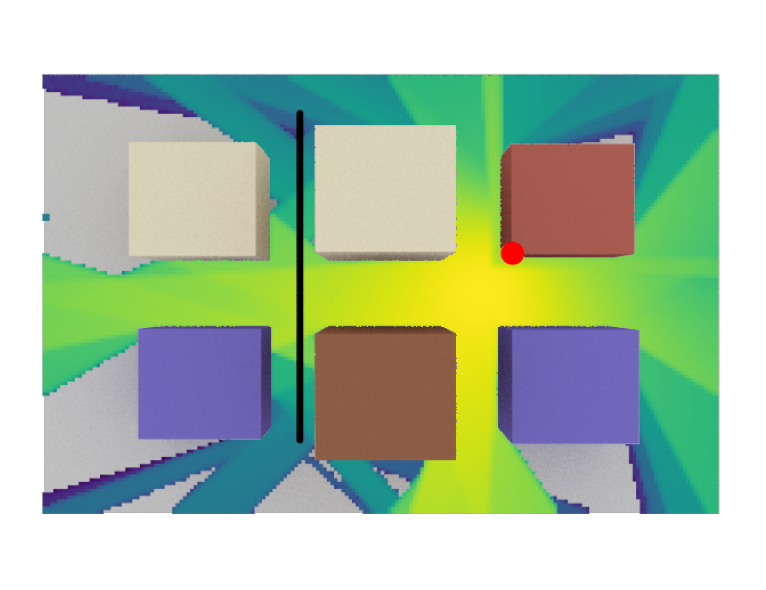
We will next show how link adaptation selects the MCS in response to the channel quality variations, while maintaining the BLER close to the target value.

The principles of link adaptation

In its general form, link adaptation (LA) accepts as input:

  • Previous HARQ feedback (ACK if the transmission was successful, else NACK);

  • Estimated channel conditions;

  • Scheduling decisions, to determine the number of coded bits;

and outputs the appropriate modulation and coding scheme (MCS), where

  • Modulation scheme determines the number of coded bits per symbol;

  • Coding scheme defines the coderate.

Note that the HARQ feedback value depends on the MCS index chosen for the last slot: the more aggressive the MCS, the higher the chance that the codeword is not correctly decoded, resulting in a negative (NACK) HARQ message.

la.png

In the following, we will create a layer-2 functionality that

  • Computes the SINR from the input channels;

  • Selects the MCS index via a general link adaptation algorithm (We will study different choices later on);

  • Generates the HARQ feedback via the PHYAbstraction functionality.

[9]:
# Initialize the PHYAbstraction object
phy_abs = PHYAbstraction()

# XLA compile for speed-ups
@tf.function(jit_compile=True)
def la_step(la,
            h,
            sinr_eff_feedback,
            harq_feedback):
    """
    Computes the SINR, select the MCS index, and generate the HARQ feedback for a
    single step of the link adaptation algorithm.
    """

    # Compute SINR
    # Note that downlink is assumed
    precoded_channel = RZFPrecodedChannel(resource_grid=resource_grid,
                                          stream_management=stream_management)
    h_eff = precoded_channel(h, tx_power=tx_power, alpha=no)

    lmmse_posteq_sinr = LMMSEPostEqualizationSINR(resource_grid=resource_grid,
                                                  stream_management=stream_management)

    # [batch_size, num_ofdm_symbols, num_effective_subcarriers, num_rx, num_streams_per_rx]
    sinr = lmmse_posteq_sinr(h_eff, no=no)[0, ...]

    # Number of allocated streams
    num_allocated_re = tf.reduce_sum(
        tf.cast(sinr > 0, tf.int32), axis=[-4, -3, -1])

    # Select MCS index via ILLA
    mcs_index = la(num_allocated_re=num_allocated_re,
                   sinr_eff=sinr_eff_feedback,
                   mcs_table_index=mcs_table_index,
                   mcs_category=1,  # downlink
                   harq_feedback=harq_feedback)

    # Send bits and collect HARQ feedback
    _, harq_feedback, sinr_eff, *_ = phy_abs(
        mcs_index,
        sinr=sinr,
        mcs_table_index=mcs_table_index,
        mcs_category=1)  # downlink

    return mcs_index, harq_feedback, sinr_eff

Next, we write the function for simulating the process defined above over multiple time steps and recording the output.

Note that we offer the option of noisy channel quality estimates.

[10]:
def run(la,
        noise_feedback=None):
    """
    Calls the link adaptation and physical abstraction blocks over multiple time
    steps and records the history of MCS indices and HARQ feedback.
    Allows for the introduction of noise in the channel estimates.
    """

    # Initialize history
    mcs_index_hist = np.zeros((num_slots))
    harq_feedback_hist = np.zeros((num_slots))
    se_la_hist = np.zeros((num_slots))
    se_shannon_hist = np.zeros((num_slots))
    sinr_eff_db_hist = np.zeros((num_slots))

    # Initialize HARQ feedback to -1 (missing)
    harq_feedback = - tf.cast(1, dtype=tf.int32)

    # Initialize SINR feedback
    sinr_eff_db_true = tf.cast([0], tf.float32)

    for i in range(num_slots):
        # [num_rx_ant, num_tx, num_tx_ant, num_ofdm_symbols, num_subcarriers]
        h = h_freq[i, ...]
        h = h[tf.newaxis, tf.newaxis, ...]
        # Noisy channel estimate
        if noise_feedback is not None:
            sinr_eff_db_feedback = sinr_eff_db_true + noise_feedback[i]
        else:
            sinr_eff_db_feedback = sinr_eff_db_true

        # Link Adaptation
        mcs_index, harq_feedback, sinr_eff_true = la_step(
            la,
            h,
            sinr_eff_feedback=db_to_lin(sinr_eff_db_feedback),
            harq_feedback=harq_feedback)
        sinr_eff_db_true = lin_to_db(sinr_eff_true)

        # Spectral efficiency
        mod_order, coderate = decode_mcs_index(
            mcs_index,
            table_index=mcs_table_index,
            is_pusch=False)

        if harq_feedback == 1:
            se_la = tf.cast(mod_order, coderate.dtype) * coderate
        else:
            se_la = tf.cast([0], tf.int32)

        # Shannon capacity
        se_shannon = log2(1 + sinr_eff_true)

        # Record history
        mcs_index_hist[i] = mcs_index[0].numpy()
        harq_feedback_hist[i] = harq_feedback[0].numpy()
        se_la_hist[i] = se_la[0].numpy()
        se_shannon_hist[i] = se_shannon[0].numpy()
        sinr_eff_db_hist[i] = sinr_eff_db_true[0].numpy()

    return sinr_eff_db_hist, mcs_index_hist, harq_feedback_hist, \
        se_la_hist, se_shannon_hist

Inner-Loop Link Adaptation (ILLA)

The simplest form of link adaptation is the so-called inner-loop link adaptation (ILLA), which selects the highest MCS whose corresponding BLER does not exceed a predefined BLER target.

Importantly, ILLA does not rely on any feedback loop, such as HARQ feedback, and fully relies on the estimated channel conditions.

illa.png

Perfect channel estimate

Next, we will run ILLA over the ray-traced scenario defined at the beginning of the notebook.

We assume that the channel estimate is perfect: ILLA observes the true effective SINR.
Clearly, this assumption is not realistic and will be lifted later on.
[11]:
# Initialize the ILLA object
illa = InnerLoopLinkAdaptation(phy_abs,
                               bler_target=bler_target)

# Simulate ILLA over multiple time steps
sinr_eff_db_hist, mcs_illa_ideal, harq_illa_ideal, se_illa_ideal, se_shannon = \
    run(illa)

We can now visualize the results:

[12]:
def plot(sinr_eff_db_hist, se_la_hist, se_shannon_hist, harq_feedback_hist,
         noise_feedback=None, fig=None, label=None, linestyle='-'):
    is_first_plot = fig is None
    if fig is not None:
        axs = fig.get_axes()
    else:
        fig, axs = plt.subplots(3, 1, sharex='col', sharey='row',
                                figsize=(5, 9))
    if is_first_plot:
        for ax in axs.flat:
            ax.yaxis.set_tick_params(labelleft=True)
            ax.xaxis.set_tick_params(labelbottom=True)
            ax.grid()

    if is_first_plot:
        axs[0].plot(sinr_eff_db_hist, label='true')
        if noise_feedback is not None:
            axs[0].plot(sinr_eff_db_hist + noise_feedback,
                        ':', label='noisy feedback')
        axs[0].set_ylabel('SINR [dB]')
        axs[0].set_xlabel('Slot')
        axs[0].legend()

    axs[1].plot(se_la_hist[:], linestyle=linestyle, label=label)
    if is_first_plot:
        axs[1].plot(se_shannon_hist, '--k', label='Shannon capacity')
    axs[1].set_ylabel('Spectral efficiency [bps/Hz]')
    axs[1].set_xlabel('Slot')
    axs[1].legend()

    if is_first_plot:
        axs[2].plot([0, num_slots - 1], [bler_target]
                    * 2, '--k', label='BLER target')
    axs[2].plot(1 - np.cumsum(harq_feedback_hist) / np.arange(1, num_slots + 1),
                linestyle=linestyle, label=label)
    axs[2].set_ylabel('Achieved BLER')
    axs[2].set_xlabel('Slot')
    axs[2].legend()
    fig.tight_layout()
    return fig, axs
[13]:
fig, axs = plot(sinr_eff_db_hist, se_illa_ideal,
                se_shannon, harq_illa_ideal, label='ILLA')
fig.suptitle('Inner Loop Link Adaptation (ILLA)\nPerfect channel estimate',
             fontsize=16, y=1)
fig.tight_layout()
plt.show()
../../_images/sys_tutorials_LinkAdaptation_28_0.png

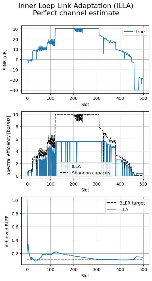
Note that the MCS evolution follows closely the one of the effective SINR: the higher the SINR, the higher the supported MCS index, hence the higher the spectral efficiency.

Moreover, the BLER is fairly close to the target.

However, the perfect channel estimate assumption is unrealistic: In real systems, the channel estimate is noisy and performed intermittently over time.

Imperfect channel estimation

We now address a more realistic scenario, where the channel estimates are noisy. We will observe that ILLA struggles in this scenario.

[14]:
noise_feedback_std = 1.5
noise_feedback = config.tf_rng.normal(
    shape=[num_slots], dtype=tf.float32, stddev=noise_feedback_std)

# Simulate ILLA over multiple time steps
sinr_eff_db_hist, mcs_illa_noisy, harq_illa_noisy, se_illa_noisy, se_shannon = \
    run(illa, noise_feedback=noise_feedback)
[15]:
fig, axs = plot(sinr_eff_db_hist, se_illa_noisy, se_shannon,
                harq_illa_noisy, noise_feedback=noise_feedback, label='ILLA')
fig.suptitle('Inner Loop Link Adaptation (ILLA)\nImperfect channel estimate',
             fontsize=16, y=1)
fig.tight_layout()
plt.show()
../../_images/sys_tutorials_LinkAdaptation_32_0.png

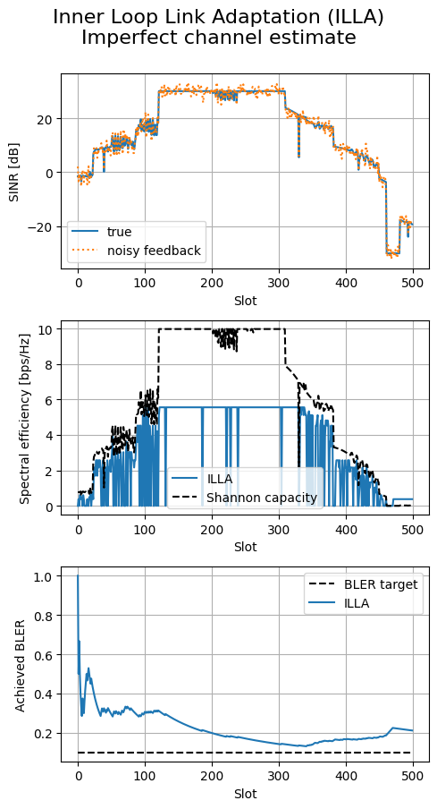
In the presence of noisy channel estimates, ILLA is no longer able to maintain the BLER close to the target value.

This is expected: ILLA fully relies on the provided estimates and does not even attempt to adjust its behavior based on the achieved BLER.

To this aim, a feedback-driven outer-loop is introduced in the following.

Outer-Loop Link Adaption (OLLA)

In contrast to ILLA, the outer-loop link adaptation (OLLA) algorithm (see [1]) introduces a simple closed-loop mechanism that adjust its behavior based on the HARQ feedback. This is realized by introducing an offset value applied to the effective SINR estimate, which varies according to the observed HARQ feedback.
Such a simple and effective mechanism enables the BLER to converge asymptotically to the predefined target value.
olla.png
[16]:
# Instantiate an OLLA object
olla = OuterLoopLinkAdaptation(phy_abs,
                               num_ut=1,
                               bler_target=bler_target)

After instantiating the OLLA object, we can now run OLLA across multiple time steps on the ray-traced scenario defined at the beginning of the notebook.

[17]:
sinr_eff_db_hist, mcs_olla, harq_olla, se_olla, se_shannon = \
    run(olla, noise_feedback=noise_feedback)

Finally, we visualize the results and compare them with ILLA.

[18]:
fig, axs = plot(sinr_eff_db_hist, se_illa_noisy, se_shannon, harq_illa_noisy,
                noise_feedback=noise_feedback, label='ILLA')
fig.suptitle('Inner Loop Link Adaptation (ILLA)\nImperfect channel estimate',
             fontsize=16, y=1)
fig, axs = plot(sinr_eff_db_hist, se_olla, se_shannon, harq_olla,
                noise_feedback=noise_feedback, fig=fig, label='OLLA', linestyle='-.')
fig.suptitle('Imperfect CQI feedback',
             fontsize=16, y=1)
fig.tight_layout()
plt.show()
../../_images/sys_tutorials_LinkAdaptation_40_0.png

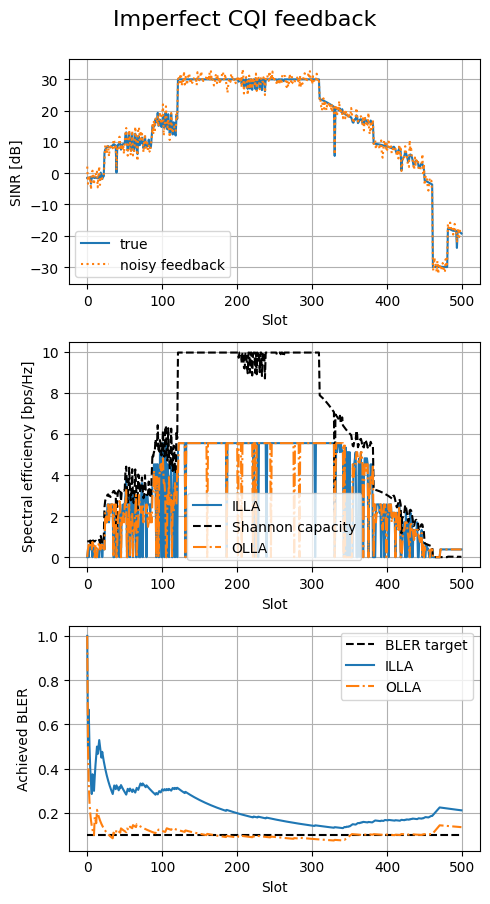
We observe that OLLA succeeds in maintaining the BLER close to the target value, although the channel estimates are noisy.

This occurs thanks to the closed-loop mechanism that adjusts the effective SINR according to the observed HARQ feedback.

Conclusions

The OuterLoopLinkAdaptation (OLLA) class adjusts the MCS index to maintain a target BLER.
By applying a feedback loop that adjusts the SINR estimate based on the observed BLER, OLLA is resilient to noisy channel quality feedback.
In contrast, InnerLoopLinkAdaptation (ILLA) lacks this robustness but serves as a key subroutine within OLLA.

References

[1] K. I. Pedersen, G. Monghal, I. Z. Kovacs, T. E. Kolding, A. Pokhariyal, F. Frederiksen, P. Mogensen. “Frequency domain scheduling for OFDMA with limited and noisy channel feedback.”,” 2007 IEEE 66th Vehicular Technology Conference, pp. 1792-1796, 2007.

Previous Next

© Copyright 2021-2025 NVIDIA CORPORATION.

Built with Sphinx using a theme provided by Read the Docs.