Proportional Fairness Scheduler

Imports
We start by importing Sionna and the relevant external libraries:
[ ]:
import os
os.environ['TF_CPP_MIN_LOG_LEVEL'] = '3'
if os.getenv("CUDA_VISIBLE_DEVICES") is None:
    gpu_num = 0 # Use "" to use the CPU
    if gpu_num!="":
        print(f'\nUsing GPU {gpu_num}\n')
    else:
        print('\nUsing CPU\n')
    os.environ["CUDA_VISIBLE_DEVICES"] = f"{gpu_num}"

# Import Sionna
try:
    import sionna.sys
except ImportError as e:
    import sys
    if 'google.colab' in sys.modules:
       # Install Sionna in Google Colab
       print("Installing Sionna and restarting the runtime. Please run the cell again.")
       os.system("pip install sionna")
       os.kill(os.getpid(), 5)
    else:
       raise e

# Configure the notebook to use only a single GPU and allocate only as much memory as needed
# For more details, see https://www.tensorflow.org/guide/gpu
import tensorflow as tf
tf.get_logger().setLevel('ERROR')
gpus = tf.config.list_physical_devices('GPU')
if gpus:
    try:
        tf.config.experimental.set_memory_growth(gpus[0], True)
    except RuntimeError as e:
        print(e)
[ ]:
# Additional external libraries
import matplotlib.pyplot as plt
import numpy as np

# Sionna components
from sionna.phy import config, Block
from sionna.phy.constants import BOLTZMANN_CONSTANT
from sionna.sys import PFSchedulerSUMIMO

# Set random seed for reproducibility
sionna.phy.config.seed = 48

# Internal computational precision
sionna.phy.config.precision = 'single'  # 'single' or 'double'
The main principle
\[\max \sum_u \log T(u).\]
To this aim, the scheduler assigns each resource \(i\) to the user with the highest PF metric, defined as the ratio of the achievable rate on resource \(i\) to the throughout achieved by the user in the past [1], [2], [3].
As a result, resources are distributed (roughly) uniformly across users, who are scheduled when their channel conditions reach a local peak.
Basic scenario
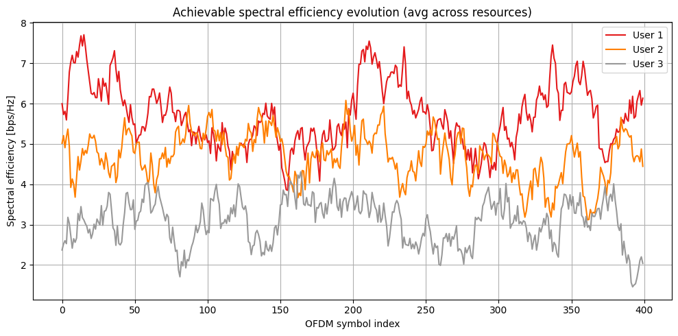
To illustrate the key principles of proportional fairness, we design a simple example where each user’s achievable rate on each subcarrier evolves according to an autoregressive (AR) process centered around a user-specific mean.
We first set the main simulation parameters:
[2]:
# Number users
num_ut = 3

# OFDM resource grid
num_subcarriers = 12
num_ofdm_symbols = 2
num_slots = 200

# User-specific average achievable rate
se_achievable_avg = config.tf_rng.uniform([num_ut], minval=1, maxval=7)

# User-specific AR multiplicative parameter
rho = config.tf_rng.uniform([num_ut], minval=0.8, maxval=.95)
Generate achievable rate time series
[3]:
class AR1(Block):
    """ Autoregressive process of order 1 for the achievable rate evolution """
    def __init__(self, mean, rho, precision=None):
        super().__init__(precision=precision)
        self.mean = tf.cast(mean, self.rdtype)
        self.rho = tf.cast(rho, self.rdtype)
        self.val = tf.Variable(mean, dtype=self.rdtype)

    def call(self):
        val_new = self.val * self.rho + self.mean * (1 - self.rho) + \
            config.tf_rng.normal(self.val.shape, dtype=self.rdtype, stddev=1)
        val_new = tf.maximum(tf.cast(0, self.rdtype), val_new)
        self.val.assign(val_new)
        return self.val
[4]:
# Broadcast across resources
se_achievable_avg = tf.tile(se_achievable_avg[tf.newaxis, :],
                            [num_subcarriers, 1])
rho = tf.tile(rho[tf.newaxis, :],
              [num_subcarriers, 1])

# Create the AR(1) process
se_achievable_ar = AR1(se_achievable_avg, rho)

# Generate the achievable rate time series
se_achievable_hist = np.zeros([num_slots*num_ofdm_symbols,
                               num_subcarriers,
                               num_ut])
for slot in range(num_slots*num_ofdm_symbols):
    se_achievable_hist[slot, :] = se_achievable_ar().numpy()
[5]:
# Create a color map or list of colors
colors = plt.cm.Set1(np.linspace(0, 1, num_ut))

# Plot
fig, ax = plt.subplots(figsize=(10, 5))
ax.set_xlabel('OFDM symbol index')
ax.set_ylabel('Spectral efficiency [bps/Hz]')
ax.set_title('Achievable spectral efficiency evolution (avg across resources)')
for ut in range(num_ut):
    # Average SE across subcarriers
    ax.plot(se_achievable_hist[..., ut].mean(axis=(-1)), color=colors[ut], label=f'User {ut+1}')
ax.legend()
ax.grid()
fig.tight_layout()
plt.show()
Schedule users
We first instantiate a PFSchedulerSUMIMO object to schedule users in a single-user MIMO system.
[6]:
# Instantiate the scheduler
scheduler = PFSchedulerSUMIMO(
    num_ut,
    num_subcarriers,
    num_ofdm_symbols,
    beta=.95)

# Use XLA compilation to speed up simulations
@tf.function(jit_compile=True)
def scheduler_xla(rate_last_slot, rate_achievable_curr):
    return scheduler(rate_last_slot, rate_achievable_curr)
The scheduler will now assign the OFDM resources to the different users according to the proportional fairness principle.
[7]:
# Initialize the achieved rate and scheduling decisions history
se_achieved_hist = np.zeros([num_slots, num_ut])
ut_scheduled_hist = np.zeros([num_slots, num_ofdm_symbols, num_subcarriers])

# Initialize the rate achieved in the last slot to 0
se_last_slot = tf.zeros([num_ut], dtype=tf.float32)

for slot in range(num_slots):
    # Extract the achievable rate in the current slot
    se_achievable_curr = se_achievable_hist[slot*num_ofdm_symbols:(slot+1)*num_ofdm_symbols, :]

    # Schedule users in the current slot across the resource grid
    # [num_ofdm_sym, num_subcarriers, num_ut, num_streams_per_ut]
    is_scheduled = scheduler(se_last_slot,
                             se_achievable_curr)

    # Sum spectral efficiency over scheduled resources in the current slot
    is_scheduled_re = tf.reduce_all(is_scheduled, axis=-1)
    se_last_slot = tf.cast(
        is_scheduled_re, se_achievable_curr.dtype) * se_achievable_curr
    # [num_ut]
    se_last_slot = tf.reduce_sum(se_last_slot, axis=[-2, -3])

    # User scheduled in each resource element
    # [num_ofdm_sym, num_subcarriers]
    ut_scheduled = tf.argmax(tf.reduce_sum(
        tf.cast(is_scheduled, tf.int32), axis=-1), axis=-1)

    # Store the results
    se_achieved_hist[slot, :] = se_last_slot.numpy()
    ut_scheduled_hist[slot, :] = ut_scheduled.numpy()

# Reshape the scheduling history
ut_scheduled_hist = np.reshape(ut_scheduled_hist,
                               [num_slots*num_ofdm_symbols, num_subcarriers])

# Per-user achieved rate
rate_achieved_pf = se_achieved_hist.sum(axis=0)
# PF metric
pf_metric_pf = np.sum(np.log(rate_achieved_pf))
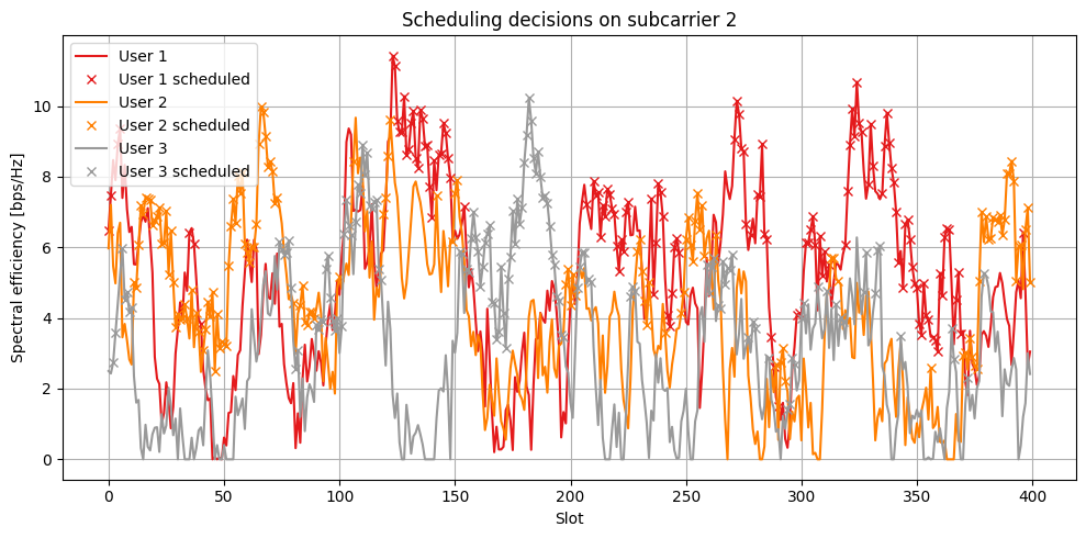
We can now visualize for a specific resource element in the grid, when a user is scheduled:
[8]:
# Select subcarrier to plot
sc = 2

# Create a color map or list of colors
colors = plt.cm.Set1(np.linspace(0, 1, num_ut))

# Plot
fig, ax = plt.subplots(figsize=(10, 5))
ax.set_xlabel('Slot')
ax.set_ylabel('Spectral efficiency [bps/Hz]')
ax.set_title(f'Scheduling decisions on subcarrier {sc}')
for ut in range(num_ut):
    # Achievable rate
    ax.plot(se_achievable_hist[:, sc, ut],
            color=colors[ut],
            label=f'User {ut+1}')
    ind_ut_scheduled = ut_scheduled_hist[:, sc] == ut
    # Scheduling decisions
    ax.plot(np.where(ind_ut_scheduled)[0],
            se_achievable_hist[ind_ut_scheduled, sc, ut],
            marker='x', color=colors[ut], linestyle='None',
            label=f'User {ut+1} scheduled')
ax.legend()
ax.grid()
fig.tight_layout()
plt.show()
We now provide an ensemble view of scheduling decisions across all subcarriers:
[9]:
show_up_to_subcarrier = 100
show_up_to_symbol = 200

cmap = plt.get_cmap('Set1', num_ut)

plt.figure(figsize=(12, 5))
plt.imshow(ut_scheduled_hist[np.arange(min(show_up_to_symbol, num_slots*num_ofdm_symbols))[:, np.newaxis],
                             np.arange(min(show_up_to_subcarrier, num_subcarriers))].T, cmap=cmap, aspect='auto')

# Add colorbar with custom ticks and labels
cbar = plt.colorbar(ticks=np.arange(num_ut))
cbar.ax.set_yticklabels([f'User {ut+1}' for ut in range(num_ut)])
cbar.set_label('User Allocation', fontsize=12)
plt.gca().invert_yaxis()
plt.xlabel('OFDM symbols')
plt.ylabel('Subcarriers')
plt.show()
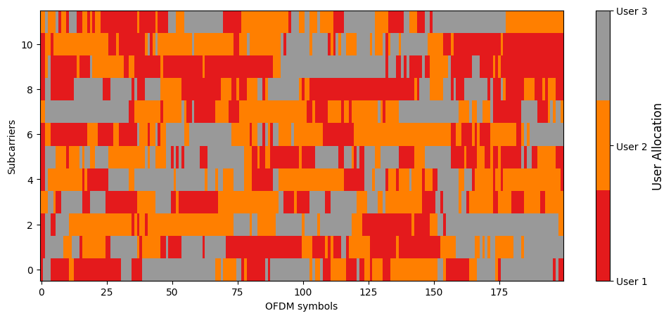
Observe that each user receives roughly the same number of resources, which is a known and desirable property of the PF scheduler.
[10]:
for ut in range(num_ut):
    perc_ut = (ut_scheduled_hist==ut).sum() / (num_ofdm_symbols*num_subcarriers*num_slots)*100
    print(f'User {ut + 1} is scheduled on {perc_ut:.2f}% of available resources')
User 1 is scheduled on 34.38% of available resources
User 2 is scheduled on 35.21% of available resources
User 3 is scheduled on 30.42% of available resources
Evaluate performance
[11]:
# Schedule users uniformly at random across the resource grid
ut_scheduled_rand_hist = config.tf_rng.uniform([num_slots*num_ofdm_symbols, num_subcarriers], minval=0, maxval=num_ut, dtype=tf.int32)
is_scheduled_rand_hist = tf.one_hot(ut_scheduled_rand_hist, num_ut, dtype=tf.float32)

rate_achieved_rand = np.sum(se_achievable_hist * is_scheduled_rand_hist.numpy(), axis=(-2,-3))

# Compute PF metric of random scheduling
pf_metric_rand = np.sum(np.log(rate_achieved_rand))

print('---------')
print('PF metric')
print('---------')
print(f'Random scheduling: {pf_metric_rand:.2f}')
print(f'PF scheduling: {pf_metric_pf:.2f}')
---------
PF metric
---------
Random scheduling: 26.55
PF scheduling: 27.65
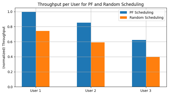
[12]:
# Data for the histogram
users = ['User 1', 'User 2', 'User 3']

# Create the histogram
fig, ax = plt.subplots(figsize=(7, 4))
bar_width = 0.25
index = np.arange(len(users))

# Normalization factor
norm_fact = max(rate_achieved_pf)
# Throughput histogram
ax.bar(index, rate_achieved_pf / norm_fact, bar_width, label='PF Scheduling')
ax.bar(index + bar_width, rate_achieved_rand / norm_fact, bar_width, label='Random Scheduling')

ax.set_ylabel('(normalized) Throughput')
ax.set_title('Throughput per User for PF and Random Scheduling')
ax.set_xticks(index + bar_width / 2)
ax.set_xticklabels(users)
ax.legend()
ax.grid()
fig.tight_layout()
plt.show()
Conclusions
The PFSchedulerSUMIMO class schedules users according the proportional fairness (PF) criterion in a single-user MIMO scenario, where at most one user can be scheduled in each resource.
By maximizing the sum of logarithms of user throughput, the PF scheduler distributes resources uniformly across users while opportunistically scheduling users when their channel conditions reach a local peak.
References
[1] A. Jalali, R. Padovani, R. Pankaj, “Data throughput of CDMA-HDR a high efficiency-high data rate personal communication wireless system.” VTC2000-Spring. 2000 IEEE 51st Vehicular Technology Conference Proceedings. Vol. 3. IEEE, 2000.
[2] A. L. Stolyar, “Maximizing queueing network utility subject to stability: Greedy primal-dual algorithm”. Queueing Systems, 50, pp. 401-457, 2005.
[3] M. Andrews, L. Qian, A. Stolyar. “Optimal utility based multi-user throughput allocation subject to throughput constraints.” Proceedings IEEE 24th Annual Joint Conference of the IEEE Computer and Communications Societies. Vol. 4. IEEE, 2005.